An introduction to genomics for programmers
About the author. Andy Thomason is the lead programmer for Genomics PLC . He has been working with graphic systems, games and compilers since the 70s; specialization - code performance.
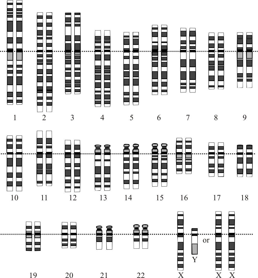
The human genome consists of two copies of approximately 3 billion base pairs of DNA, which are encoded using the letters A, C, G and T. This is about two bits for each base pair:
3,000,000,000 × 2 × 2/8 = 1,500,000,000 or about 1.5 GB of data.
')
In fact, these copies are very similar, and the DNA of all people is almost the same: from merchants from Wall Street to Australian Aborigines.
There are a number of “reference genomes,” such as Ensembl Fasta files . Reference genomes help build a map with specific characteristics that are present in human DNA, but not unique to specific people.
For example, we can determine the “location” of a gene that encodes a BRCA2 protein that is responsible for DNA repair in breast cancer: this gene .
It is located on chromosome 13, from position 32315474 to 32400266.
People are so similar that for the representation of a person it is usually enough to store a small set of “variations”.
Over time, our DNA is damaged by cosmic rays and copying errors, so the DNA that parents transmit to children is slightly different from their own.
The recombination mixes the genes even more, so the child’s DNA inherits from each parent a mixture of the grandparents' DNA from this side.
Therefore, for each change in our DNA, it is enough to keep only the differences from the reference genome. Usually they are saved in a VCF (Variant Call Format) file.
Like almost all files in bioinformatics, it is a file of type TSV (text format with tabs).
You can get your own VCF file from companies like 23 and Me and Ancestry.com : pay relatively little money and send a sample that is sequenced on a DNA microchip. It highlights fragments where DNA corresponds to the expected sequences.
An abbreviated example of the VCF specifications :
Here we have three people named NA00001, NA00002 and NA00003 (we are very serious about the security of personal data in the world of genetics), who in position 14370 of chromosome 20 have certain differences
There are two numbers per person, since we all have two copies of chromosome 20 (one from each parent; the only exception is the sex chromosome). I was not lucky that I have only one X chromosome, so I inherited color blindness from my grandfather through my mother).
Such options are possible:
VCF files are considered “phased” if you can figure out which particular chromosome the variant is on or at least where it is located relative to its neighbors. In practice, it is difficult to say which chromosome DNA came from, so you have to speculate!
Thus, we have a bit vector
Using this bit vector, we can try to figure out which parts of the genome affect diseases or other individual properties, such as hair color or growth. For each option, we build a haplotype for the measured traits ( phenotype ).
GWAS (Genome wide association study, polygenomic search for associations) is the basis for genetic analysis of variants. He compares variations with observational data.
For example:
Please note that each has two haplotypes, because we have a pair of chromosomes.
Here we see that options 1 are associated with higher growth, and the values correspond to linear regression:
In practice, the data is really a lot of noise, and the error is usually larger than the
The easiest way to regress is to apply the Moore-Penrose inversion .
We compose a 2 × 2 covariance matrix with the scalar product of two vectors, and we solve the problem using the least squares method.
We have trillions of data points, so it’s important to do this effectively.
Since we inherit large fragments of the genome from our parents, certain areas of DNA look very similar: they are much more similar than the case dictates.
This is good for us, because genes continue to work in the same way as their ancestors, but badly for genomics researchers. This means that the differences are not enough to determine the variations that caused a change in the phenotype.
Non-equilibrium adhesion (LD) determines how similar the two vectors are with variations.
It calculates a value between -1 and 1, where
To determine the similarity of variations, we create large square LD matrices for specific places in the genome. In practice, many of the variations around this place are almost identical to the variant in the middle.
The matrix looks something like this, with large squares of similarity.
Real values are not 0 or 1, but very similar.
A recombination occurred between v7 and v8. Because of this, v0..v7 is different from v8..vg.
The problem of similarity is that we know that one of the options in the group caused something, but we do not know which one.
This limits the resolution of our genomic microscope , and to solve the problem will have to use additional methods such as functional genomics.
In the end, you can never be 100% sure which particular region of the genome caused a particular individual feature, this is the essence of genetics. Biology is not an exact machine with perfect factory-made parts. This is a boiling mass of accidents that somehow create what we call life. That is why statistics, or “machine learning,” is so important, as it is now fashionable to call it.
Genes: a brief introduction
The human genome consists of two copies of approximately 3 billion base pairs of DNA, which are encoded using the letters A, C, G and T. This is about two bits for each base pair:
3,000,000,000 × 2 × 2/8 = 1,500,000,000 or about 1.5 GB of data.
')
In fact, these copies are very similar, and the DNA of all people is almost the same: from merchants from Wall Street to Australian Aborigines.
There are a number of “reference genomes,” such as Ensembl Fasta files . Reference genomes help build a map with specific characteristics that are present in human DNA, but not unique to specific people.
For example, we can determine the “location” of a gene that encodes a BRCA2 protein that is responsible for DNA repair in breast cancer: this gene .
It is located on chromosome 13, from position 32315474 to 32400266.
Genetic variations
People are so similar that for the representation of a person it is usually enough to store a small set of “variations”.
Over time, our DNA is damaged by cosmic rays and copying errors, so the DNA that parents transmit to children is slightly different from their own.
The recombination mixes the genes even more, so the child’s DNA inherits from each parent a mixture of the grandparents' DNA from this side.
Therefore, for each change in our DNA, it is enough to keep only the differences from the reference genome. Usually they are saved in a VCF (Variant Call Format) file.
Like almost all files in bioinformatics, it is a file of type TSV (text format with tabs).
You can get your own VCF file from companies like 23 and Me and Ancestry.com : pay relatively little money and send a sample that is sequenced on a DNA microchip. It highlights fragments where DNA corresponds to the expected sequences.
An abbreviated example of the VCF specifications :
  ## fileDate = 20090805
 ## source = myImputationProgramV3.1
 ## reference = 1000GenomesPilot-NCBI36
 ## phasing = partial
 #CHROM POS ID REF ALT QUAL FILTER INFO FORMAT NA00001 NA00002 NA00003
 20 14370 rs6054257 GA 29 PASS NS = 3; DP = 14; AF = 0.5; DB; H2 GT: GQ: DP: HQ 0 | 0: 48: 1: 51.51 1 | 0: 48: 8: 51.51 1/1: 43: 5:.,.
Here we have three people named NA00001, NA00002 and NA00003 (we are very serious about the security of personal data in the world of genetics), who in position 14370 of chromosome 20 have certain differences
0|0 , 1|0 and 1|1 from G to A.There are two numbers per person, since we all have two copies of chromosome 20 (one from each parent; the only exception is the sex chromosome). I was not lucky that I have only one X chromosome, so I inherited color blindness from my grandfather through my mother).
Such options are possible:
  0 | 0 both chromosomes correspond to the reference sample
 1 | 0 and 0 | 1 only one chromosome is different from the standard
 1 | 1 both chromosomes are different from the standard
VCF files are considered “phased” if you can figure out which particular chromosome the variant is on or at least where it is located relative to its neighbors. In practice, it is difficult to say which chromosome DNA came from, so you have to speculate!
Thus, we have a bit vector
001011 , which is enough to classify three people in this variation. These are haplotypes or variations of individual chromosomes.GWAS research
Using this bit vector, we can try to figure out which parts of the genome affect diseases or other individual properties, such as hair color or growth. For each option, we build a haplotype for the measured traits ( phenotype ).
GWAS (Genome wide association study, polygenomic search for associations) is the basis for genetic analysis of variants. He compares variations with observational data.
For example:
  Haplotype Height Person
 0 1.5m NA00001
 0 1.5m
 1 1.75m NA00002
 0 1.75m
 1 1.95m NA00003
 1 1.95m
Please note that each has two haplotypes, because we have a pair of chromosomes.
Here we see that options 1 are associated with higher growth, and the values correspond to linear regression:
  beta Growth variation with variation variation.
 standard error Error rate.
In practice, the data is really a lot of noise, and the error is usually larger than the
beta , but often we have several options, where beta much higher than the error. This relationship — the Z-score and its associated p-value — indicates which options are most likely to affect growth.The easiest way to regress is to apply the Moore-Penrose inversion .
We compose a 2 × 2 covariance matrix with the scalar product of two vectors, and we solve the problem using the least squares method.
We have trillions of data points, so it’s important to do this effectively.
Curse of disequilibrium clutch
Since we inherit large fragments of the genome from our parents, certain areas of DNA look very similar: they are much more similar than the case dictates.
This is good for us, because genes continue to work in the same way as their ancestors, but badly for genomics researchers. This means that the differences are not enough to determine the variations that caused a change in the phenotype.
Non-equilibrium adhesion (LD) determines how similar the two vectors are with variations.
It calculates a value between -1 and 1, where
  -1 Completely opposite variations.
  0 Variations are not similar.
  1 The variations are exactly the same.
To determine the similarity of variations, we create large square LD matrices for specific places in the genome. In practice, many of the variations around this place are almost identical to the variant in the middle.
The matrix looks something like this, with large squares of similarity.
  v0 v2 v4 v6 v8 va vc ve vg
       v1 v3 v5 v7 v9 vb vd vf
 v0 1 1 1 1 1 1 1 1 0 0 0 0 0 0 0 0
 v1 1 1 1 1 1 1 1 1 0 0 0 0 0 0 0 0
 v2 1 1 1 1 1 1 1 1 0 0 0 0 0 0 0 0
 v3 1 1 1 1 1 1 1 1 0 0 0 0 0 0 0 0
 v4 1 1 1 1 1 1 1 1 0 0 0 0 0 0 0 0
 v5 1 1 1 1 1 1 1 1 0 0 0 0 0 0 0 0
 v6 1 1 1 1 1 1 1 1 0 0 0 0 0 0 0 0
 v7 1 1 1 1 1 1 1 1 0 0 0 0 0 0 0 0
 v8 0 0 0 0 0 0 0 0 1 1 1 1 1 1 1 1
 v9 0 0 0 0 0 0 0 0 1 1 1 1 1 1 1 1
 va 0 0 0 0 0 0 0 0 1 1 1 1 1 1 1 1
 vb 0 0 0 0 0 0 0 0 1 1 1 1 1 1 1 1
 vc 0 0 0 0 0 0 0 0 1 1 1 1 1 1 1 1
 vd 0 0 0 0 0 0 0 0 1 1 1 1 1 1 1 1
 ve 0 0 0 0 0 0 0 0 1 1 1 1 1 1 1 1
 vf 0 0 0 0 0 0 0 0 1 1 1 1 1 1 1 1
 vg 0 0 0 0 0 0 0 0 1 1 1 1 1 1 1 1
Real values are not 0 or 1, but very similar.
A recombination occurred between v7 and v8. Because of this, v0..v7 is different from v8..vg.
The problem of similarity is that we know that one of the options in the group caused something, but we do not know which one.
This limits the resolution of our genomic microscope , and to solve the problem will have to use additional methods such as functional genomics.
Conclusion
In the end, you can never be 100% sure which particular region of the genome caused a particular individual feature, this is the essence of genetics. Biology is not an exact machine with perfect factory-made parts. This is a boiling mass of accidents that somehow create what we call life. That is why statistics, or “machine learning,” is so important, as it is now fashionable to call it.
Source: https://habr.com/ru/post/452622/
All Articles