MIMO spatial diversity: Alamouti, DET and other spatial diversity

To transmit a message from a base station to a mobile device (and vice versa), an electromagnetic wave has to overcome a significant number of obstacles: reflections, refractions, scattering, shading, Doppler frequency shifts, and so on. First, it is accepted to call all these effects multiplicative (from the English. Multiplication - multiplication) - according to the mathematical model of such effects. And, secondly, it can be collected under the general term fading .

From standard to standard, from generation to generation, from technology to technology, scientists and engineers have struggled and are struggling with the problem of fading mitigation.

And some solutions are widespread. Let's say more: almost all of them, one way or another, are connected with the concept of diversity (diversity) .

Source of illustration (no, this is not advertising, just a good combination of the desired term and a cat).

An example of such solutions:

Frequency hopping - against frequency selective fading;
Channel estimation and equalization through GSM feedback to suppress changes in the time domain;
Spread Spectrum (UMTS);
Pilot signals (starting from UMTS) downstream (Down-link) and tracking (signal tracking) upstream (Up-link) - to suppress changes in the time domain;
OFDM - LTE, against frequency selective fading;
Temporal spacing ( robust coding );
Polarization spacing (on the transmitter side) + Adders (combiners, on the receiver side);
Spatial separation .

The last of the mentioned techniques we will consider today in the framework of another topic on MIMO .

Space diversity order and array gain

The first.

There is such a concept - the order of spatial diversity (space diversity order): if the same information can be collected from different directions , then the hope to restore it will increase correctly. As an example of life, you can provide a collection of information about the same event from independent sources of informers. In radio communication, we can increase this order, including by applying MISO , SIMO or MIMO .

The theoretical limit of such diversity M_TM_R where M_T - the number of transmit antennas, and M_R - the number of receiving antennas. Remember this.

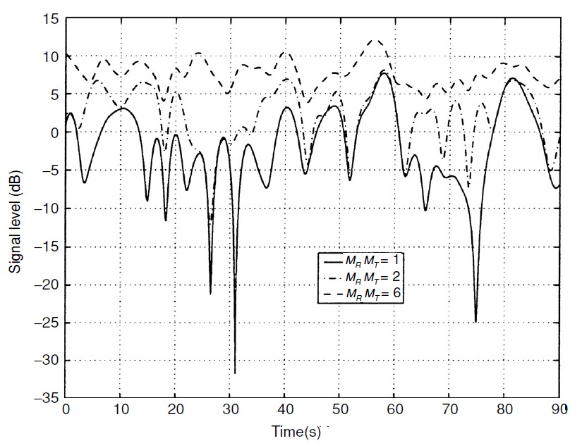
Fig.1. Channel stability caused by an increase in the order of spatial diversity. At values $M_TM_R \ to \ infty$ the channel is completely stabilized and turns into a channel without fading (AWGN) [1, p.101] .

The second.

Using SIMO , MIMO and even MISO (in the case of a known channel), you can get the so-called array gain . This means that using multiple receiving antennas and / or correct energy distribution on the transmitting side allows you to increase the signal-to-noise ratio (SNR) - and thus reduce the number of errors.

The orders of diversity and gain of the array for different configurations can be derived analytically [1, c. 86 - 100] and summarized in one table [1, p. 101] and for the case when the channel is unknown (CU - Channel Unknown), and for the case when the channel is known (CK - Channel Known) on the transmitter side.

Configuration	Diversity order	Array gain
SIMO (CU, Rx-MRC)
SIMO (CK, Rx-MRC)
MISO (CU, OSTBC)		one
MISO (CK, Tx-MRC)
MIMO (CU, OSTBC)
MIMO (CK, DET)

Okay, albeit in broad strokes, but now we have at least some understanding of the theoretical aspects of the suppression of fading. The next question is how to reach these theoretical limits? What are the activation techniques for the considered winnings?

Decision number 1. Space Time Codes

One of the most popular classes of spatial diversity solutions is, perhaps, the space-time code class. For example, I know the Alamouti method, familiar to many (block code example) [2, c. 40-46]:

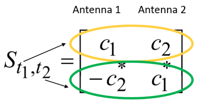
Where c_i at i = 1,2 - these are some input characters, t_i at i = 1,2 - These are time counts (time slots), and $\ mathbf {s}$ - this is, in fact, the coding matrix.

The Alamouti circuit is orthogonal [1, pp.93-95, 97-98] and, most importantly, does not require Channel State Information.

A mathematical description of the transmission of the Alamouti-encoded signal, as well as several examples of modeling this technique in MatLab can be found in my repository . Interested welcome!

However, as you can see, the Alamouti circuit is a case where we only have two transmit antennas ( M_T = 2 ).
But do not lose heart ahead of time: other options are available, of course, they are just called a little differently. For example, according to [3], the following coding schemes can be applied:

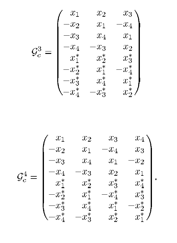
Fig. 2. Transmission schemes for cases and [2].

And many other options: just to meet the conditions of orthogonality.

For such codes, the same procedures for encoding and decoding are required as for the Alamouti code. Therefore, they are usually united under the general term orthogonal space-time block codes (OSTBC - Ortogonal Space-Time Block Codes).

Much attention is paid to this class of codes in the “Introduction to MIMO Systems” materials from MathWorks. I strongly advise all interested to read!

What's the price?

As can be seen from the transmission scheme, although we transmit characters in parallel, we spend several time slots on it. Consequently, we are sacrificing bandwidth (at a minimum, losing it). For the Alamouti scheme, such a compromise is symmetrical: we use 2 antennas and 2 time slots (as if using SISO in terms of throughput). Other schemes may affect the transfer rate even more.

Decision number 2. DET: Dominant Eigenmode Transmission

Well, for the previous class of technician, knowledge about the channel was not important to us. But what if we still have this knowledge? Is there a more suitable technique in this case?

In one of my previous articles, we discussed that, having knowledge of the state of the channel, we can apply various signal processing methods to increase the throughput. The same principle also works to improve noise immunity.

Probably, many have heard about the MRC method and many know that this method is most appropriate for the SIMO case, when there is only one antenna at the transmission, but there are many at the reception, which means there is something to combine.

But, probably, already a smaller number of readers encountered the MRC on the transmission side (Tx-MRC) [1, p. 95.96], and even less with DET technology (Dominant Eigenmode Transmission) [1, p. 98-100]. Fix it!

To begin, consider the general case of the MIMO channel and the last of these methods - DET.

What is the essence:

If the transmitter has a matrix $\ mathbf {H}$ then it can be processed.
For example, decompose it via SVD : $\ mathbf {H} = \ mathbf {U} \ mathbf {\ Sigma} \ mathbf {V} ^ H$ , thus obtaining several matrices of a certain property.
These properties can be used to optimize transmission, for example, by applying pre-coding.

We introduce some pre-coding vector:

$\ underset {M_T \ times1} {\ mathbf {w}} = \ sqrt {M_T} \ underset {M_T \ times1} {\ mathbf {v} _1}$

Where $\ mathbf {v} _1$ - this is the first (dominant, so to speak) matrix vector $\ mathbf {V}$ .

Moreover, we can also record the post-processing vector:

$\ underset {M_R \ times1} {\ mathbf {g}} = \ underset {M_R \ times1} {\ mathbf {u} _1}$

Where $\ mathbf {u} _1$ Is the first matrix vector $\ mathbf {U}$ .

Redefine the received signal model (see bandwidth topic ):

${z} = \ underset {1 \ times M_R} {\ mathbf {g} ^ H} \ underset {M_R \ times 1} {\ mathbf {y}} = \ mathbf {g} ^ H \ sqrt {\ frac { E_s} {M_T}} \ mathbf {H} \ mathbf {w} s + \ mathbf {g} ^ H \ mathbf {n} = \ sqrt {E_s} \ mathbf {u} _1 ^ H \ mathbf {H} \ mathbf {v} _1 s + \ hat {\ mathbf {n}} = \ sqrt {E_s} \ sigma_ {max} s + \ hat {\ mathbf {n}}$

Voila! The magic of linear algebra singled out the most profitable among all paths of propagation and sent all the energy there. In fact, we have a linear beamforming algorithm.

The price of the considered approach is the same, as in the case of OSTBC, throughput limiting. True, this is happening now especially in the spatial domain.

Why does the method contain in its name eigenvalues (eigen values), if we talked only about singular values?

Because the eigenvalues (power of propagation paths - fading) can be directly derived from singular numbers (amplitudes of fading):

$\ mathbf {R} _ {\ mathbf {HH} ^ H} = \ mathbf {HH} ^ H = \ mathbf {Q} \ mathbf {\ Lambda} \ mathbf {Q} ^ H = \ mathbf {Q} \ begin {bmatrix} \ lambda_ {max} & & & & \\ &. & & & \\ & &. & & \\ & & &. & \\ & & & & \ lambda_ {min} \\ \ end {bmatrix} \ mathbf {Q} ^ H$

Well, with DET it is more or less clear - what about Tx-MRC?

It's still easier with him - this is a special case of DET, and now we will prove it.

For Tx-MRC, the following pre-coding vector has been proposed in the literature:

$\ mathbf {w} = \ sqrt {M_T} \ frac {\ mathbf {h} ^ H} {\ sqrt {|| \ mathbf {h} || ^ 2_F}}$

We keep in mind that the square of the Frobenius norm is equal to the eigenvalue and, accordingly, to the square of the singular number $|| \ mathbf {h} || ^ 2_F = \ lambda_ {max} = \ sigma ^ 2_ {max}$ (in the case of SIMO and MISO).

Then redefine the received signal model, only for the MISO case:

$y = \ sqrt {\ frac {E_s} {M_T}} \ mathbf {h} \ mathbf {w} s + \ mathbf {n} = \ sqrt {\ frac {E_s} {M_T}} \ mathbf {h} \ sqrt {M_T} \ frac {\ mathbf {h} ^ H} {\ sqrt {|| \ mathbf {h} || ^ 2_F}} s + \ mathbf {n}} = \ frac {\ sqrt {E_s}} {\ sigma_ {max}} \ mathbf {h} \ mathbf {h} ^ H s + \ mathbf {n}} = \ frac {\ sqrt {E_s}} {\ sigma_ {max}} || \ mathbf {h } || _F ^ 2 s + \ mathbf {n}} = \ frac {\ sqrt {E_s}} {\ sigma_ {max}} \ lambda_ {max} s + \ mathbf {n}} = \ sqrt {E_s} \ sigma_ {max} s + \ mathbf {n}}$

Q.E.D.

Notice, now we are not just talking about the diversity of signals on the transmitting side and combining them on the receiving side, as was the case with OSTBC. Now we are talking about the optimal distribution of energy. This means that the values of array gain in this case are higher than those of OSTBC.

Now that all the words have been spoken, we will try to model our techniques.

Modeling

Today I read a bit: for the OSTBC modeling, ready-made objects from Communication Toolbox (MatLab R2014a - which one was) were used:

comm.OSTBCEncoder - Ortogonal Space-Time Block Codes Encoder;
comm.OSTBCCombiner - Ortogonal Space-Time Block Codes Combiner.

For modulation and demodulation (and BER counting), not objects, but functions were used. Their analogues are in the Octave communications package.

Source codes can be viewed here.

clear all; close all; clc snapshots = 100000; EbNo = 0:15; M = 2; % modulation order (BPSK) Mt = 2; % num. of Tx antennas Mr = [1; 2]; % num. of Rx antennas ostbcEnc = comm.OSTBCEncoder('NumTransmitAntennas', Mt); % for Alamouti ric_ber = zeros(length(EbNo), length(M), length(Mr)); sum_BER_alam = zeros(length(EbNo), length(M), length(Mr)); sum_BER_det = zeros(length(EbNo), length(M), length(Mr)); for mr = 1:length(Mr) ostbcComb = comm.OSTBCCombiner('NumTransmitAntennas', Mt, 'NumReceiveAntennas', Mr(mr)); H = zeros(Mr(mr), Mt, snapshots); alam_fad_msg = zeros(snapshots, Mr(mr)); for m = 1:length(M) ric_ber(:,m,mr) = berfading(EbNo, 'psk', M(m), Mr(mr)*Mt, 0); snr = EbNo+10*log10(log2(M(m))); % Signal-to-Noise Ratio message = randi([0, M(m)-1],100000,1); mod_msg = pskmod(message, M(m), 0, 'gray'); Es = mean(abs(mod_msg).^2); % symbol energy alam_msg = step(ostbcEnc, mod_msg); % OSTBC encoding % Channel h = (1/sqrt(2))*(randn(Mr(mr),Mt,snapshots/Mt)... + 1j*randn(Mr(mr),Mt, snapshots/Mt)); % Rayleigh flat fading % Channel is stable during to time-slots: H(:,:,1:2:end-1) = h; H(:,:,2:2:end) = h; pathGainself = permute(H,[3,2,1]); % Transmit through the channel (Alamouti): for q = 1:snapshots; alam_fad_msg(q,:) = (sqrt(Es/Mt)*H(:,:,q)*alam_msg(q,:).').'; end % DET: sigmas = zeros(length(mod_msg), 1); for hi = 1:length(mod_msg) [U, Sigma, Vh] = svd(H(:, :, hi)); sigmas(hi) = Sigma(1, 1); end det_fad_msg = mod_msg.*sigmas; No = Es./((10.^(EbNo./10))*log2(M(m))); % Noise spectrum density for c = 1:500 for jj = 1:length(EbNo) alam_noisy_msg = alam_fad_msg + ... sqrt(No(jj)/2)*(randn(size(alam_fad_msg)) + ... 1j*randn(size(alam_fad_msg))); % AWGN alam_decodeData = step(ostbcComb,alam_noisy_msg,pathGainself); %OSTBC combining alam_demod_msg = pskdemod(alam_decodeData, M(m), 0, 'gray'); % demodulation [number,alam_BER(c,jj)] = biterr(message, alam_demod_msg); % BER det_noisy_msg = det_fad_msg+ ... sqrt(No(jj)/2)*(randn(size(mod_msg)) + ... 1j*randn(size(mod_msg))); %AWGN det_decodeData = det_noisy_msg./sigmas; % Zero-Forcing equalization det_demod_msg = pskdemod(det_decodeData, M(m), 0, 'gray'); % demodulation [number,det_BER(c,jj)] = biterr(message, det_demod_msg); % BER end end sum_BER_alam(:,m, mr) = sum(alam_BER)./c; sum_BER_det(:,m, mr) = sum(det_BER)./c; end end figure(1) semilogy(EbNo, sum_BER_alam(:, 1, 1), 'b-o', ... EbNo, sum_BER_det(:,1,1), 'b->',... EbNo, ric_ber(:,1,1), 'b-',... EbNo, sum_BER_alam(:, 1, 2), 'r-o', ... EbNo, sum_BER_det(:,1,2), 'r->',... EbNo, ric_ber(:,1,2), 'r-',... 'LineWidth', 1.5) title('BPSK (Rayleigh flat fading)') legend('Alamouti (2x1)','Tx-MRC (2x1)','2-nd order diversity', ... 'Alamouti (2x2)','DET (2x2)','4-th order diversity') xlabel('EbNo (dB)') ylabel('BER') grid on

It should be something like this:

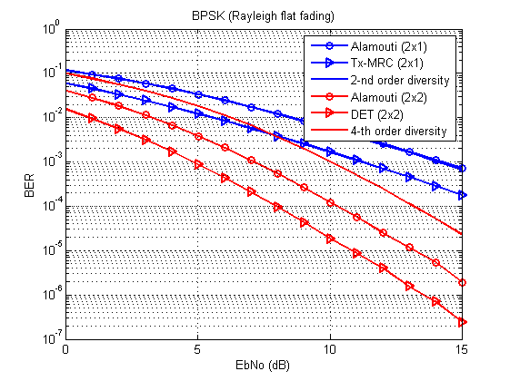
Fig. 3. Bit / Character Error Curves for Different Transmission Techniques (BPSK, Rayleigh Flat Fading Channel). Compare with [1, p. 96, 100].

And now the question is: where is the curve of the theoretical second-order separation boundary?

Answer

Everything is according to the table: this curve completely coincides with Alamouti 2x1. In the case of MIMO, the array gain also comes into play, and therefore the curves are split.

One way or another, DET (or Tx-MRC) is expectedly ahead of Alamouti in quality.

Like this: knowledge is power!

Literature

Paulraj, Arogyaswami, Rohit Nabar, and Dhananjay Gore. Introduction to space-time wireless communications. Cambridge university press, 2003.
Bakulin M. G., Varukina L. A., Kreyndelin V. B. MIMO technology: Principles and Algorithms // M .: Hotline – Telecom. - 2014. - T. 244.
Tarokh, V., Jafarkhani, H., & Calderbank, AR (1999). Space-time block codes from orthogonal designs. IEEE Transactions on Information theory, 45 (5), 1456-1467.

I give my greetings to the faculty and student fraternity of my native specialty !

Source: https://habr.com/ru/post/452494/

All Articles