My numerical test of the “Absolute Course” hypothesis
Hi, Habr!
I found this publication interesting: We obtain absolute rates from paired cross-exchange rates and I wanted to check the possibility of finding this aaa absolute exchange rate through numerical simulation, having completely abandoned linear algebra.
')
The results were interesting.
The experiment will be small: 4 currencies, 6 currency pairs. For each pair, one dimension course.
The hypothesis is that the value of any currency can be expressed by some value that will take into account the value of other currencies in which it is quoted, despite the fact that other currencies themselves will be expressed in the value of all other currencies. This is an interesting recursive task.
There are 4 currencies:
For them, currency pairs were recruited:
Please note that if the number of currencies n = 4, then the number of pairs k = (n ^ 2 - n) / 2 = 6. It makes no sense to look for usdeur, if eurusd is quoted ...
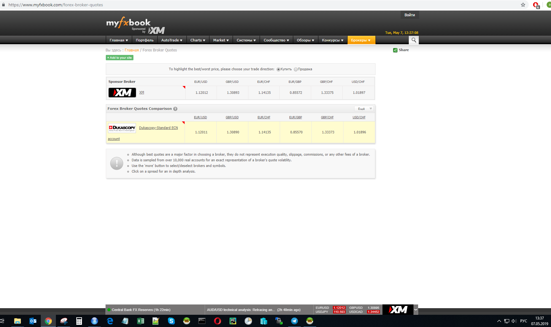
At time t, the exchange rate of one of the providers was measured:
Calculations will be made for these values.
I solve the problem, analytically taking the gradient of the loss function, which in essence is a system of equations.
The experiment code will be in R:
R allows using the function stats :: D to take the derivative of a function. For example, if we want to differentiate the USD currency, we get the following expression:
The gradient step will be controlled by the lr parameter and all of this is taken with a negative sign.
That is, in human words, we select the rates of 4 currencies so that all currency pairs in the experiment get values equal to the initial values of these pairs. Mmm, let's solve the puzzle - in the forehead!
In order not to stretch, I will immediately inform you of the following: the experiment as a whole was a success, the code worked, the error went very close to zero. But then I noticed that the results are always different.
A question for connoisseurs: it looks like this task has an unlimited number of solutions, but in this I am a complete zero, I think, I will be told in the comments.
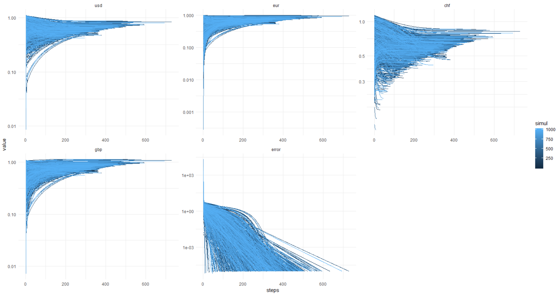
To verify the (in) stability of the solution, I conducted a simulation 1000 times without fixing the PRNG LED for the starting values of the currency values.
And here comes a picture from the kata: error reaches 0.00001 and less (optimization is set this way) always, with the values of currencies flooding away — he knows where. It turns out, always a different solution, gentlemen!
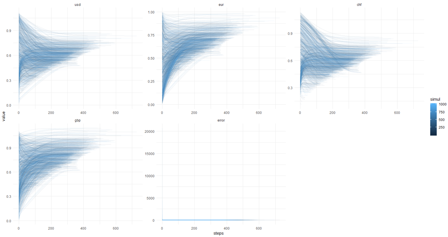
Once again this picture, y-axis in original units (not a log.):
So that you can repeat this, below I enclose the full code.
The code for 1000 simulations runs for about a minute.
That's what remains for me is not clear:
The whole idea seems very vague in the absence of any intelligible assumptions and restrictions. But it was interesting!
Well, I also wanted to say that you can do without the MNC, when the data is tricky, the matrices are singular, well, or when the theory is not well known (ehh ...).
Thank you eavprog for the initial message.
Until!
I found this publication interesting: We obtain absolute rates from paired cross-exchange rates and I wanted to check the possibility of finding this aaa absolute exchange rate through numerical simulation, having completely abandoned linear algebra.
')
The results were interesting.
The experiment will be small: 4 currencies, 6 currency pairs. For each pair, one dimension course.
So, let's begin
The hypothesis is that the value of any currency can be expressed by some value that will take into account the value of other currencies in which it is quoted, despite the fact that other currencies themselves will be expressed in the value of all other currencies. This is an interesting recursive task.
There are 4 currencies:
- usd
- eur
- chf
- gbp
For them, currency pairs were recruited:
- eurusd
- gbpusd
- eurchf
- eurgbp
- gbpchf
- usdchf
Please note that if the number of currencies n = 4, then the number of pairs k = (n ^ 2 - n) / 2 = 6. It makes no sense to look for usdeur, if eurusd is quoted ...
At time t, the exchange rate of one of the providers was measured:
Calculations will be made for these values.
Maths
I solve the problem, analytically taking the gradient of the loss function, which in essence is a system of equations.
The experiment code will be in R:
#set.seed(111) usd <- runif(1) eur <- runif(1) chf <- runif(1) gbp <- runif(1) # snapshot of values at time t eurusd <- 1.12012 gbpusd <- 1.30890 eurchf <- 1.14135 eurgbp <- 0.85570 gbpchf <- 1.33373 usdchf <- 1.01896 ## symbolic task ------------ express <- expression( (eurusd - eur / usd) ^ 2 + (gbpusd - gbp / usd) ^ 2 + (eurchf - eur / chf) ^ 2 + (eurgbp - eur / gbp) ^ 2 + (gbpchf - gbp / chf) ^ 2 + (usdchf - usd / chf) ^ 2 ) eval(express) x = 'usd' D(express, x) eval(D(express, x)) R allows using the function stats :: D to take the derivative of a function. For example, if we want to differentiate the USD currency, we get the following expression:
2 * (eur / usd ^ 2 * (eurusd - eur / usd)) + 2 * (gbp / usd ^ 2 * (gbpusd -To reduce the value of the express function, we will perform a gradient descent and it is immediately clear (we see square differences) that the minimum value will be zero, which is what we need.
gbp / usd)) - 2 * (1 / chf * (usdchf - usd / chf))
-deriv_vals * lr The gradient step will be controlled by the lr parameter and all of this is taken with a negative sign.
That is, in human words, we select the rates of 4 currencies so that all currency pairs in the experiment get values equal to the initial values of these pairs. Mmm, let's solve the puzzle - in the forehead!
results
In order not to stretch, I will immediately inform you of the following: the experiment as a whole was a success, the code worked, the error went very close to zero. But then I noticed that the results are always different.
A question for connoisseurs: it looks like this task has an unlimited number of solutions, but in this I am a complete zero, I think, I will be told in the comments.
To verify the (in) stability of the solution, I conducted a simulation 1000 times without fixing the PRNG LED for the starting values of the currency values.
And here comes a picture from the kata: error reaches 0.00001 and less (optimization is set this way) always, with the values of currencies flooding away — he knows where. It turns out, always a different solution, gentlemen!
Once again this picture, y-axis in original units (not a log.):
So that you can repeat this, below I enclose the full code.
Code
# clear environment rm(list = ls()); gc() ## load libs library(data.table) library(ggplot2) library(magrittr) ## set WD -------------------------------- # your dir here ... ## set vars ------------- currs <- c( 'usd', 'eur', 'chf', 'gbp' ) ############ ## RUN SIMULATION LOOP ------------------------------- simuls <- 1000L simul_dt <- data.table() for( s in seq_len(simuls) ) { #set.seed(111) usd <- runif(1) eur <- runif(1) chf <- runif(1) gbp <- runif(1) # snapshot of values at time t eurusd <- 1.12012 gbpusd <- 1.30890 eurchf <- 1.14135 eurgbp <- 0.85570 gbpchf <- 1.33373 usdchf <- 1.01896 ## symbolic task ------------ express <- expression( (eurusd - eur / usd) ^ 2 + (gbpusd - gbp / usd) ^ 2 + (eurchf - eur / chf) ^ 2 + (eurgbp - eur / gbp) ^ 2 + (gbpchf - gbp / chf) ^ 2 + (usdchf - usd / chf) ^ 2 ) ## define gradient and iterate to make descent to zero -------------- iter_max <- 1e+3 lr <- 1e-3 min_tolerance <- 0.00001 rm(grad_desc_func) grad_desc_func <- function( lr, curr_list ) { derivs <- character(length(curr_list)) deriv_vals <- numeric(length(curr_list)) grads <- numeric(length(curr_list)) # symbolic derivatives derivs <- sapply( curr_list, function(x){ D(express, x) } ) # derivative values deriv_vals <- sapply( derivs, function(x){ eval(x) } ) # gradient change values -deriv_vals * lr } ## get gradient values ---------- progress_list <- list() for( i in seq_len(iter_max) ) { grad_deltas <- grad_desc_func(lr, curr_list = currs) currency_vals <- sapply( currs , function(x) { # update currency values current_val <- get(x, envir = .GlobalEnv) new_delta <- grad_deltas[x] if(new_delta > -1 & new_delta < 1) { new_delta = new_delta } else { new_delta = sign(new_delta) } new_val <- current_val + new_delta if(new_val > 0 & new_val < 2) { new_val = new_val } else { new_val = current_val } names(new_val) <- NULL # change values of currencies by gradient descent step in global env assign(x, new_val , envir = .GlobalEnv) # save history of values for later plotting new_val } ) progress_list[[i]] <- c( currency_vals, eval(express) ) if( eval(express) < min_tolerance ) { break('solution was found') } } ## check results ---------- # print( # paste0( # 'Final error: ' # , round(eval(express), 5) # ) # ) # # print( # round(unlist(mget(currs)), 5) # ) progress_dt <- rbindlist( lapply( progress_list , function(x) { as.data.frame(t(x)) } ) ) colnames(progress_dt)[length(colnames(progress_dt))] <- 'error' progress_dt[, steps := 1:nrow(progress_dt)] progress_dt_melt <- melt( progress_dt , id.vars = 'steps' , measure.vars = colnames(progress_dt)[colnames(progress_dt) != 'steps'] ) progress_dt_melt[, simul := s] simul_dt <- rbind( simul_dt , progress_dt_melt ) } ggplot(data = simul_dt) + facet_wrap(~ variable, scales = 'free') + geom_line( aes( x = steps , y = value , group = simul , color = simul ) ) + scale_y_log10() + theme_minimal() The code for 1000 simulations runs for about a minute.
Conclusion
That's what remains for me is not clear:
- Is it possible to stabilize the solution in a clever mathematical way?
- will convergence with a greater number of currencies and currency pairs;
- if stability cannot be, then for each new snapshot of data our currencies will walk as they please, if you do not fix the PRNG seat, and this is a failure.
The whole idea seems very vague in the absence of any intelligible assumptions and restrictions. But it was interesting!
Well, I also wanted to say that you can do without the MNC, when the data is tricky, the matrices are singular, well, or when the theory is not well known (ehh ...).
Thank you eavprog for the initial message.
Until!
Source: https://habr.com/ru/post/450874/
All Articles