Understanding the FFT algorithm
Hello, friends. Tomorrow the course “Algorithms for Developers” starts, and we have only one unpublished translation left. Actually we correct and share with you the material. Go.
Fast Fourier Transform (FFT) is one of the most important signal processing and data analysis algorithms. I used it for years, without having formal knowledge in the field of computer science. But this week it occurred to me that I never wondered how the FFT computes the discrete Fourier transform so quickly. I shook off the dust from the old book on algorithms, opened it, and read with pleasure about the deceptively simple computational trick that J.W. Cooley and John Tukey described in their classic 1965 work on this topic.

')
The purpose of this post is to plunge into the Kuli-Tukey FFT algorithm, explaining the symmetries that lead to it, and show a few simple implementations in Python that apply the theory in practice. I hope that this study will give data analysts, like me, a more complete picture of what is going on under the hood of our algorithms.
Discrete Fourier Transform
FFT is fast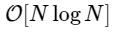 algorithm to calculate the discrete fourier transform (DFT), which is directly calculated for
  . The DFT, like the more familiar continuous version of the Fourier transform, has a direct and inverse form, which are defined as follows:
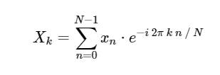
Direct Discrete Fourier Transform (DFT):
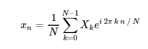
Inverse Discrete Fourier Transform (IDFT):
Conversion from
Due to the importance of the FFT (hereinafter the equivalent FFT - Fast Fourier Transform can be used) in many areas of Python contains many standard tools and wrappers for its calculation. Both NumPy and SciPy have shells from the extremely well-tested FFTPACK library, which are found in the
For now, however, let's leave these implementations aside and ask ourselves how we can calculate the FFT in Python from scratch.
Discrete Fourier Transform Calculation
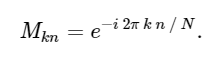
For simplicity, we will deal only with the direct transformation, since the inverse transformation can be implemented in a very similar way. Looking at the above DFT (DFT) expression, we see that this is nothing more than a straight-line linear operation: multiplying a matrix by a vector

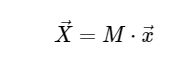
with matrix M given
With this in mind, we can calculate the DFT using simple matrix multiplication as follows:
In [1]:
We can double-check the result by comparing it with the built-in Numpy FFT function:
In [2]:
0ut [2]:
Just to confirm the slowness of our algorithm, we can compare the execution time of these two approaches:
In [3]:
We are more than 1000 times slower, which is to be expected for such a simplified implementation. But this is not the worst. For an input vector of length N, the FFT algorithm is scaled as , while our slow algorithm scales as
  . That means for
  elements, we expect the FFT to complete in about 50 ms, while our slow algorithm takes about 20 hours!
So how does the FFT achieve such acceleration? The answer is to use symmetry.
Symmetries in the discrete Fourier transform
One of the most important tools in the construction of algorithms is the use of problem symmetries. If you can analytically show that one part of the problem is simply related to the other, you can calculate the sub-result only once and save these computational costs. Coulee and Tukey used this approach to obtain FFT.
We will begin with a question about the meaning . From our expression above:

where we used the identity exp [2π in] = 1, which holds for any integer n.
The last line shows the DFT symmetry property well:
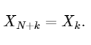
Simple extension
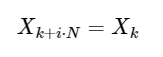
for any integer i. As we will see below, this symmetry can be used to calculate the DFT much faster.
DFT in FFT: the use of symmetry
Cooley and Tukey showed that it is possible to divide the FFT calculations into two smaller parts. From the definition of DFT we have:
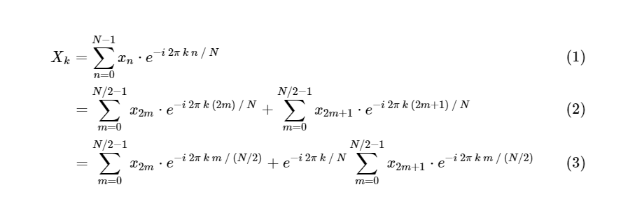
We divided one discrete Fourier transform into two terms, which themselves are very similar to smaller discrete Fourier transforms, one to values with an odd number and one to values with an even number. However, so far we have not saved any computational cycles. Each term consists of (N / 2) ∗ N calculations, total .
.
The trick is to use symmetry in each of these conditions. Since the range of k is 0≤k <N, and the range of n is 0≤n <M≡N / 2, we see from the symmetry properties above that we need to perform only half of the calculations for each subtask. Our calculation became
  where M is two times less than N.
But there is no reason to dwell on this: as long as our smaller Fourier transforms have an even M, we can reapply this divide-and-conquer approach, each time halving the computational cost, until our arrays are small enough so that the strategy no longer promises any benefits. In the asymptotic limit, this recursive approach scales as O [NlogN].
This recursive algorithm can be very quickly implemented in Python, starting from our slow DFT code, when the size of the subtask becomes small enough:
In [4]:
Here we will make a quick check that our algorithm gives the correct result:
In [5]:
Out [5]:
Let us compare this algorithm with our slower version:
-In [6]:
Our calculation is faster than the direct version in order! Moreover, our recursive algorithm is asymptotically : we implemented a fast Fourier transform.
Please note that we are still not close to the speed of the embedded FFT algorithm in numpy, and this is to be expected. The FFTPACK algorithm behind
A good strategy for speeding up your code when working with Python / NumPy is to vectorize repetitive calculations whenever possible. This we can do - in the process of deleting our recursive function calls, which will make our Python FFT even more efficient.
Vectorized Numpy-version
Note that in the above recursive FFT implementation at the lowest recursion level, we perform N / 32 identical matrix-vector products. The effectiveness of our algorithm will benefit if we simultaneously compute these matrix-vector products as a single matrix-matrix product. At each subsequent level of recursion, we also perform repetitive operations that can be vectorized. NumPy does an excellent job with this operation, and we can use this fact to create this vectorized version of the fast Fourier transform:
In [7]:
Although the algorithm is a bit more opaque, it is simply a permutation of the operations used in the recursive version, with one exception: we use symmetry in the calculation of the coefficients and build only half of the array. Again, we confirm that our function gives the correct result:
In [8]:
Out [8]:
As our algorithms become much more efficient, we can use a larger array to compare the time, leaving
In [9]:
We have improved our implementation by an order of magnitude! Now we are at a distance of about 10 times from the standard FFTPACK, using only a couple dozen lines of pure Python + NumPy. Although this is still not computationally relevant, in terms of readability, the Python version is far superior to the FFTPACK source code, which you can view here .
So how does FFTPACK achieve this last acceleration? Well, basically, this is just a matter of detailed accounting. FFTPACK spends a lot of time reusing any intermediate calculations that can be reused. Our ragged version still includes an excess of memory allocation and copying; in a low-level language such as Fortran, it is easier to control and minimize memory usage. In addition, the Cooley-Tukey algorithm can be extended to use partitions with a size other than 2 (what we have implemented here is known as the Cooley-Tukey Radix FFT on the basis of 2). Other more complex FFT algorithms can also be used, including fundamentally different approaches based on convolutional data (see, for example, Bluustein's algorithm and Raider's algorithm). The combination of the above extensions and methods can lead to very fast FFT even on arrays whose size is not a power of two.
Although pure Python functions are probably useless in practice, I hope they have some insight into what is happening against the background of FFT-based data analysis. As data specialists, we can cope with the implementation of the “black box” of fundamental tools created by our more algorithmic colleagues, but I firmly believe that the more we understand about low-level algorithms that we apply to our data, the best practices we will.
This post was completely written in IPython Notepad. The complete notebook can be downloaded here or viewed statically here .
Many may notice that the material is far from new, but it seems to us that it is quite relevant. In general, write whether the article was useful. We are waiting for your comments.
Fast Fourier Transform (FFT) is one of the most important signal processing and data analysis algorithms. I used it for years, without having formal knowledge in the field of computer science. But this week it occurred to me that I never wondered how the FFT computes the discrete Fourier transform so quickly. I shook off the dust from the old book on algorithms, opened it, and read with pleasure about the deceptively simple computational trick that J.W. Cooley and John Tukey described in their classic 1965 work on this topic.
')
The purpose of this post is to plunge into the Kuli-Tukey FFT algorithm, explaining the symmetries that lead to it, and show a few simple implementations in Python that apply the theory in practice. I hope that this study will give data analysts, like me, a more complete picture of what is going on under the hood of our algorithms.
Discrete Fourier Transform
FFT is fast
algorithm to calculate the discrete fourier transform (DFT), which is directly calculated for . The DFT, like the more familiar continuous version of the Fourier transform, has a direct and inverse form, which are defined as follows:Direct Discrete Fourier Transform (DFT):
Inverse Discrete Fourier Transform (IDFT):
Conversion from
xn → Xk is a transfer from configuration space to frequency space and can be very useful both for studying the power spectrum of a signal and for converting certain tasks for more efficient computation. Some examples of this in action can be found in Chapter 10 of our future book on astronomy and statistics, where you can also find images and source code in Python. An example of using the FFT to simplify the integration of complex otherwise differential equations, see my post “Solving the Schrödinger equation in Python” .Due to the importance of the FFT (hereinafter the equivalent FFT - Fast Fourier Transform can be used) in many areas of Python contains many standard tools and wrappers for its calculation. Both NumPy and SciPy have shells from the extremely well-tested FFTPACK library, which are found in the
numpy.fft and scipy.fftpack sub- numpy.fft , respectively. The fastest FFT that I know about is in the FFTW package, which is also available in Python through the PyFFTW package.For now, however, let's leave these implementations aside and ask ourselves how we can calculate the FFT in Python from scratch.
Discrete Fourier Transform Calculation
For simplicity, we will deal only with the direct transformation, since the inverse transformation can be implemented in a very similar way. Looking at the above DFT (DFT) expression, we see that this is nothing more than a straight-line linear operation: multiplying a matrix by a vector
with matrix M given
With this in mind, we can calculate the DFT using simple matrix multiplication as follows:
In [1]:
import numpy as np def DFT_slow(x): """Compute the discrete Fourier Transform of the 1D array x""" x = np.asarray(x, dtype=float) N = x.shape[0] n = np.arange(N) k = n.reshape((N, 1)) M = np.exp(-2j * np.pi * k * n / N) return np.dot(M, x) We can double-check the result by comparing it with the built-in Numpy FFT function:
In [2]:
x = np.random.random(1024) np.allclose(DFT_slow(x), np.fft.fft(x)) 0ut [2]:
TrueJust to confirm the slowness of our algorithm, we can compare the execution time of these two approaches:
In [3]:
%timeit DFT_slow(x) %timeit np.fft.fft(x) 10 loops, best of 3: 75.4 ms per loop 10000 loops, best of 3: 25.5 µs per loop We are more than 1000 times slower, which is to be expected for such a simplified implementation. But this is not the worst. For an input vector of length N, the FFT algorithm is scaled as
, while our slow algorithm scales as . That means for elements, we expect the FFT to complete in about 50 ms, while our slow algorithm takes about 20 hours!So how does the FFT achieve such acceleration? The answer is to use symmetry.
Symmetries in the discrete Fourier transform
One of the most important tools in the construction of algorithms is the use of problem symmetries. If you can analytically show that one part of the problem is simply related to the other, you can calculate the sub-result only once and save these computational costs. Coulee and Tukey used this approach to obtain FFT.
We will begin with a question about the meaning
. From our expression above:where we used the identity exp [2π in] = 1, which holds for any integer n.
The last line shows the DFT symmetry property well:
Simple extension
for any integer i. As we will see below, this symmetry can be used to calculate the DFT much faster.
DFT in FFT: the use of symmetry
Cooley and Tukey showed that it is possible to divide the FFT calculations into two smaller parts. From the definition of DFT we have:
We divided one discrete Fourier transform into two terms, which themselves are very similar to smaller discrete Fourier transforms, one to values with an odd number and one to values with an even number. However, so far we have not saved any computational cycles. Each term consists of (N / 2) ∗ N calculations, total
.The trick is to use symmetry in each of these conditions. Since the range of k is 0≤k <N, and the range of n is 0≤n <M≡N / 2, we see from the symmetry properties above that we need to perform only half of the calculations for each subtask. Our calculation
became where M is two times less than N.But there is no reason to dwell on this: as long as our smaller Fourier transforms have an even M, we can reapply this divide-and-conquer approach, each time halving the computational cost, until our arrays are small enough so that the strategy no longer promises any benefits. In the asymptotic limit, this recursive approach scales as O [NlogN].
This recursive algorithm can be very quickly implemented in Python, starting from our slow DFT code, when the size of the subtask becomes small enough:
In [4]:
def FFT(x): """A recursive implementation of the 1D Cooley-Tukey FFT""" x = np.asarray(x, dtype=float) N = x.shape[0] if N % 2 > 0: raise ValueError("size of x must be a power of 2") elif N <= 32: # this cutoff should be optimized return DFT_slow(x) else: X_even = FFT(x[::2]) X_odd = FFT(x[1::2]) factor = np.exp(-2j * np.pi * np.arange(N) / N) return np.concatenate([X_even + factor[:N / 2] * X_odd, X_even + factor[N / 2:] * X_odd]) Here we will make a quick check that our algorithm gives the correct result:
In [5]:
x = np.random.random(1024) np.allclose(FFT(x), np.fft.fft(x)) Out [5]:
TrueLet us compare this algorithm with our slower version:
-In [6]:
%timeit DFT_slow(x) %timeit FFT(x) %timeit np.fft.fft(x) 10 loops, best of 3: 77.6 ms per loop 100 loops, best of 3: 4.07 ms per loop 10000 loops, best of 3: 24.7 µs per loop Our calculation is faster than the direct version in order! Moreover, our recursive algorithm is asymptotically
: we implemented a fast Fourier transform.Please note that we are still not close to the speed of the embedded FFT algorithm in numpy, and this is to be expected. The FFTPACK algorithm behind
fft numpy is a Fortran implementation that has received years of refinements and optimizations. In addition, our NumPy solution includes both the recursion of the Python stack and the allocation of many temporary arrays, which increases computation time.A good strategy for speeding up your code when working with Python / NumPy is to vectorize repetitive calculations whenever possible. This we can do - in the process of deleting our recursive function calls, which will make our Python FFT even more efficient.
Vectorized Numpy-version
Note that in the above recursive FFT implementation at the lowest recursion level, we perform N / 32 identical matrix-vector products. The effectiveness of our algorithm will benefit if we simultaneously compute these matrix-vector products as a single matrix-matrix product. At each subsequent level of recursion, we also perform repetitive operations that can be vectorized. NumPy does an excellent job with this operation, and we can use this fact to create this vectorized version of the fast Fourier transform:
In [7]:
def FFT_vectorized(x): """A vectorized, non-recursive version of the Cooley-Tukey FFT""" x = np.asarray(x, dtype=float) N = x.shape[0] if np.log2(N) % 1 > 0: raise ValueError("size of x must be a power of 2") # N_min here is equivalent to the stopping condition above, # and should be a power of 2 N_min = min(N, 32) # Perform an O[N^2] DFT on all length-N_min sub-problems at once n = np.arange(N_min) k = n[:, None] M = np.exp(-2j * np.pi * n * k / N_min) X = np.dot(M, x.reshape((N_min, -1))) # build-up each level of the recursive calculation all at once while X.shape[0] < N: X_even = X[:, :X.shape[1] / 2] X_odd = X[:, X.shape[1] / 2:] factor = np.exp(-1j * np.pi * np.arange(X.shape[0]) / X.shape[0])[:, None] X = np.vstack([X_even + factor * X_odd, X_even - factor * X_odd]) return X.ravel() Although the algorithm is a bit more opaque, it is simply a permutation of the operations used in the recursive version, with one exception: we use symmetry in the calculation of the coefficients and build only half of the array. Again, we confirm that our function gives the correct result:
In [8]:
x = np.random.random(1024) np.allclose(FFT_vectorized(x), np.fft.fft(x)) Out [8]:
TrueAs our algorithms become much more efficient, we can use a larger array to compare the time, leaving
DFT_slow :In [9]:
x = np.random.random(1024 * 16) %timeit FFT(x) %timeit FFT_vectorized(x) %timeit np.fft.fft(x) 10 loops, best of 3: 72.8 ms per loop 100 loops, best of 3: 4.11 ms per loop 1000 loops, best of 3: 505 µs per loop We have improved our implementation by an order of magnitude! Now we are at a distance of about 10 times from the standard FFTPACK, using only a couple dozen lines of pure Python + NumPy. Although this is still not computationally relevant, in terms of readability, the Python version is far superior to the FFTPACK source code, which you can view here .
So how does FFTPACK achieve this last acceleration? Well, basically, this is just a matter of detailed accounting. FFTPACK spends a lot of time reusing any intermediate calculations that can be reused. Our ragged version still includes an excess of memory allocation and copying; in a low-level language such as Fortran, it is easier to control and minimize memory usage. In addition, the Cooley-Tukey algorithm can be extended to use partitions with a size other than 2 (what we have implemented here is known as the Cooley-Tukey Radix FFT on the basis of 2). Other more complex FFT algorithms can also be used, including fundamentally different approaches based on convolutional data (see, for example, Bluustein's algorithm and Raider's algorithm). The combination of the above extensions and methods can lead to very fast FFT even on arrays whose size is not a power of two.
Although pure Python functions are probably useless in practice, I hope they have some insight into what is happening against the background of FFT-based data analysis. As data specialists, we can cope with the implementation of the “black box” of fundamental tools created by our more algorithmic colleagues, but I firmly believe that the more we understand about low-level algorithms that we apply to our data, the best practices we will.
This post was completely written in IPython Notepad. The complete notebook can be downloaded here or viewed statically here .
Many may notice that the material is far from new, but it seems to us that it is quite relevant. In general, write whether the article was useful. We are waiting for your comments.
Source: https://habr.com/ru/post/449996/
All Articles