Adaptive antenna arrays: how does it work? (Basics)
The last few years I have devoted to the study and creation of various algorithms for the spatial processing of signals in adaptive antenna arrays, and I continue to do this as part of my work now. Here I would like to share the knowledge and chips that I discovered. I hope that it will be useful for people starting out to study this area of signal processing or just interested.
What is an adaptive antenna array?
An antenna array is a set of antenna elements that are arranged in some way in space. Simplified structure of an adaptive antenna array, which we will consider, can be represented as follows:
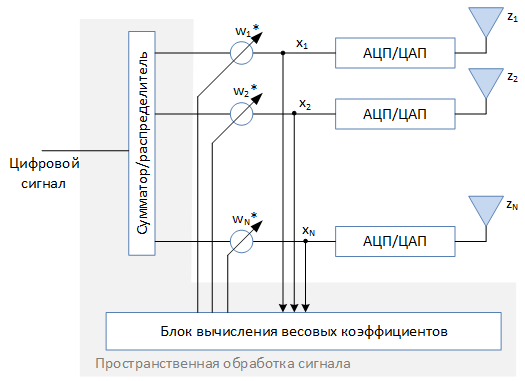
Adaptive antenna arrays are not rarely called “smart” antennas ( Smart antenna ). The “smart” antenna array is made by the spatial signal processing unit and the algorithms implemented in it. These algorithms analyze the received signal and form a set of weights. $ inline $ w_1 ... w_N $ inline $ which determine the amplitude and initial phase of the signal for each of the elements. The specified amplitude-phase distribution determines the radiation pattern of the entire lattice as a whole. The ability to synthesize the radiation pattern of the required form and change it during signal processing is one of the main features of adaptive antenna arrays, allowing to solve a wide range of tasks . But first things first.
')
How is the radiation pattern formed?
The radiation pattern characterizes the signal power emitted in a certain direction. For simplicity, let the lattice elements be isotropic, i.e. for each of them, the power of the emitted signal does not depend on the direction. Amplification or attenuation of the power emitted by the grating in a certain direction is obtained due to the interference of the electromagnetic wave emitted by different elements of the antenna array. A stable interference pattern for EMW is possible only under the condition of their coherence , i.e. the phase difference of the signals should not change with time. In the ideal case, each of the elements of the antenna array should emit a harmonic signal at the same carrier frequency $ inline $ f_ {0} $ inline $ . However, in practice, one has to work with narrowband signals having a spectrum of finite width $ inline $ \ Delta f << f_ {0} $ inline $ .
Let all elements of the AR emit the same signal with a complex amplitude. $ inline $ x_n (t) = u (t) $ inline $ . Then at the remote receiver, the signal received from the nth element can be represented in an analytical form:
$$ display $$ a_n (t) = u (t- \ tau_n) e ^ {i2 \ pi f_0 (t- \ tau_n)} $$ display $$
Where $ inline $ \ tau_n $ inline $ - delay in the propagation of the signal from the antenna element to the point of reception.Such a signal is “quasi-harmonic,” and to satisfy the coherence condition, it is necessary that the maximum delay in the propagation of the electromagnetic wave between any two elements be much less than the characteristic time of change in the signal envelope. $ inline $ t $ inline $ i.e. $ inline $ u (t- \ tau_n) ≈ u (t- \ tau_m) $ inline $ . Thus, the condition on the coherence of a narrowband signal can be written as follows:
$$ display $$ T≈ \ frac {1} {\ Delta f} >> \ frac {D_ {max}} {c} = max (\ tau_k- \ tau_m) $$ display $$
Where $ inline $ D_ {max} $ inline $ - the maximum distance between the elements of the AR , and $ inline $ with $ inline $ - the speed of light.When receiving a signal, coherent summation is performed in a digital form in the spatial processing unit. In this case, the complex value of the digital signal at the output of this block is determined by the expression:
$$ display $$ y = \ sum_ {n = 1} ^ Nw_n ^ * x_n $$ display $$
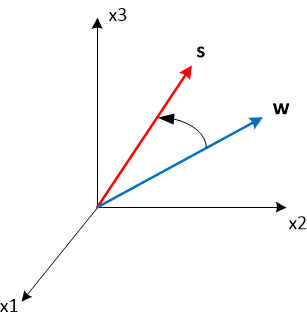
It is more convenient to present the last expression in the form of the scalar product of N-dimensional complex vectors in matrix form:$$ display $$ y = (\ textbf {w}, \ textbf {x}) = \ textbf {w} ^ H \ textbf {x} $$ display $$
where w and x are column vectors, and $ inline $ (.) ^ H $ inline $ - Hermitian conjugation operation.The vector representation of signals is one of the basic when working with antenna arrays, since often avoids cumbersome mathematical calculations. In addition, identification of a signal received at a certain time with a vector often allows one to abstract from a real physical system and to understand what exactly is happening from the point of view of geometry.
In order to calculate the radiation pattern of the antenna array, it is necessary to mentally and consistently “launch” onto it a set of plane waves from all possible directions. In this case, the values of the elements of the vector x can be represented as follows:
$$ display $$ x_n = s_n = \ exp \ {- i (\ textbf {k} (\ phi, \ theta), \ textbf {r} _n) \} $$ display $$
where k is the wave vector , $ inline $ \ phi $ inline $ and $ inline $ \ theta $ inline $ - azimuth angle and elevation angle , characterizing the direction of arrival of a plane wave, $ inline $ \ textbf {r} _n $ inline $ - coordinate of the antenna element, $ inline $ s_n $ inline $ - an element of the phasing vector s of a plane wave with a wave vector k (in the English-language literature, the phasing vector is called the steerage vector). The dependence of the square amplitude of y on $ inline $ \ phi $ inline $ and $ inline $ \ theta $ inline $ determines the radiation pattern of the antenna array at the reception for a given weight vector w .Features of the antenna array
It is convenient to investigate the general properties of the radiation pattern of antenna arrays conveniently on a linear equidistant antenna array in a horizontal plane (that is, the radiation pattern depends only on the azimuth angle $ inline $ \ phi $ inline $ ). Convenient from two points of view: analytical calculations and visual presentation.
Calculate the DN for the unit weight vector ( $ inline $ w_n = 1, n = 1 ... N $ inline $ ), following the above approach.
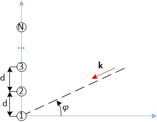
The projection of the wave vector on the vertical axis: $ inline $ k_v = - \ frac {2 \ pi} {\ lambda} \ sin \ phi $ inline $
The vertical coordinate of the antenna element with the index n: $ inline $ r_ {nv} = (n-1) d $ inline $
Here d is the period of the antenna array (the distance between adjacent elements), λ is the wavelength. All other elements of the vector r are equal to zero.
The signal received by the antenna array is recorded as follows:
$$ display $$ y = \ sum_ {n = 1} ^ {N} 1 ⋅ \ exp \ {i2 \ pi n \ frac {d} {\ lambda} \ sin \ phi \} $$ display $$
Let us apply the formula for the sum of a geometric progression and the representation of trigonometric functions through complex exponentials :$$ display $$ y = \ frac {1- \ exp \ {i2 \ pi N \ frac {d} {\ lambda} \ sin \ phi \}} {1- \ exp \ {i2 \ pi \ frac {d } {\ lambda} \ sin \ phi \}} = \ frac {\ sin (\ pi \ frac {Nd} {\ lambda} \ sin \ phi)} {\ sin (\ pi \ frac {d} {\ lambda } \ sin \ phi)} \ exp \ {i \ pi \ frac {d (N-1)} {\ lambda} \ sin \ phi \} $$ display $$
As a result, we get:
$$ display $$ F (\ phi) = | y | ^ 2 = \ frac {\ sin ^ 2 (\ pi \ frac {Nd} {\ lambda} \ sin \ phi)} {\ sin ^ 2 (\ pi \ frac {d} {\ lambda} \ sin \ phi)} $$ display $$
Radiation pattern frequency
The resulting antenna pattern is a periodic function of the sine of the angle. This means that for certain values of the d / λ ratio, it has diffraction (additional) maxima.

The position of "diffractionary" can be viewed directly from the formula for DN. However, we will try to understand where they come from physically and geometrically (in N-dimensional space).
Elements of the phasing vector s are complex exponents $ inline $ e ^ {i \ Psin} $ inline $ whose values are determined by the value of the generalized angle $ inline $ \ Psi = 2 \ pi \ frac {d} {\ lambda} \ sin \ phi $ inline $ . If there are two generalized angles corresponding to different directions of arrival of a plane wave, for which $ inline $ \ Psi_1 = \ Psi_2 + 2 \ pi m $ inline $ , it means two things:
- Physically: the plane wave fronts coming from these directions induce identical amplitude-phase distributions of electromagnetic oscillations on the elements of the antenna array.
- Geometrically: the phasing vectors for these two directions are the same.
Connected in a similar way the direction of arrival of the waves are from the point of view of the antenna array equivalent and not distinguishable among themselves.
How to determine the area of the corners, in which only one main maximum of the bottoms always lies? We will do this in the vicinity of the zero azimuth from the following considerations: the magnitude of the phase shift between two adjacent elements must lie in the interval from $ inline $ - \ pi $ inline $ before $ inline $ \ pi $ inline $ .
$$ display $$ - \ pi <2 \ pi \ frac {d} {\ lambda} \ sin \ phi <\ pi $$ display $$
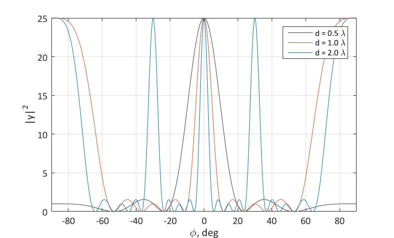
Solving this inequality we obtain the condition on the domain of uniqueness in a neighborhood of zero:$$ display $$ | \ sin \ phi | <\ frac {\ lambda} {2d} $$ display $$
It can be seen that the size of the region of single-valuedness by the angle depends on the ratio d / λ . If d = 0.5 λ , then each direction of signal arrival is “individually”, and the area of unambiguity covers the full range of angles. If d = 2.0 λ , then the directions 0, ± 30, ± 90 are equivalent. Diffraction lobes appear on the directivity pattern.
Typically, diffraction lobes tend to be suppressed using directional antenna elements. In this case, the complete radiation pattern of the antenna array is the product of the DN of one element and the grid of isotropic elements. The parameters of the DN of one element are usually chosen based on the condition on the region of uniqueness of the antenna array.
Main petal width
An engineering formula for estimating the width of the main lobe of an antenna system is widely known : $ inline $ \ Delta \ phi ≈ \ frac {\ lambda} {D} $ inline $ where D is the characteristic size of the antenna. The formula is used for various types of antennas, including mirror ones. We show that it is also valid for antenna arrays.
Let us determine the width of the main lobe with the first zeros of the DN in the vicinity of the main maximum. Expression numerator for $ inline $ F (\ phi) $ inline $ vanishes at $ inline $ \ sin \ phi = m \ frac {\ lambda} {dN} $ inline $ . The first zeros correspond to m = ± 1. Putting $ inline $ \ frac {\ lambda} {dN} << 1 $ inline $ we get $ inline $ \ Delta \ phi = 2 \ frac {\ lambda} {dN} $ inline $ .
Typically, the width of the pattern of the AR directivity is determined by the level of half power (-3 dB). In this case, use the expression:
$$ display $$ \ Delta \ phi≈0.88 \ frac {\ lambda} {dN} $$ display $$

The width of the main lobe can be controlled by setting different amplitudes for the weights of the antenna array. Consider three distributions:
- Uniform amplitude distribution (weights 1): $ inline $ w_n = 1 $ inline $ .
- Amplitude values (weights 2) falling to the edges of the grid: $ inline $ w_n = 0.5 + 0.3 \ cos (2 \ pi \ frac {n-1} {N} - \ pi \ frac {N-1} {N}) $ inline $
- The amplitude values (weights 3) increasing towards the edges of the grid: $ inline $ w_n = 0.5-0.3 \ cos (2 \ pi \ frac {n-1} {N} - \ pi \ frac {N-1} {N}) $ inline $
The figure shows the resulting normalized radiation patterns on a logarithmic scale:
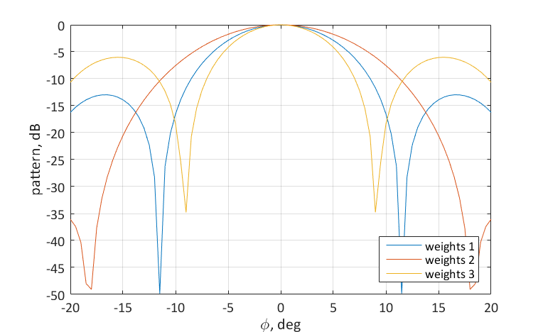
The following tendencies can be traced from the figure: the distribution of the amplitudes of the weight coefficients falling to the edges of the lattice leads to a broadening of the main lobe of the DN, but a decrease in the level of side lobes. The amplitude values increasing towards the edges of the antenna array, on the contrary, lead to a narrowing of the main lobe and an increase in the level of the side panels. Here it is convenient to consider the limiting cases:
- The amplitudes of the weight coefficients of all elements, except the extreme ones, are zero. Weights for extreme elements are equal to one. In this case, the lattice becomes equivalent to a two-element AP with a period D = (N-1) d . It is not difficult to estimate the width of the main lobe using the formula given above. At the same time, the side panels will turn into diffraction peaks and level with the main maximum.
- The weight of the central element is equal to one, and all the rest is zero. In this case, we got essentially one antenna with an isotropic radiation pattern.
Head High Direction
So, we looked at how to adjust the width of the main lobe of the DN AR . Now let's see how to steer the direction. Recall the vector expression for the received signal. Suppose we want the maximum of the radiation pattern to look in a certain direction. $ inline $ \ phi_0 $ inline $ . This means that from this direction should be taken maximum power. This direction corresponds to the phasing vector $ inline $ \ textbf {s} (\ phi_0) $ inline $ in the N- dimensional vector space, and the received power is defined as the square of the scalar product of this phasing vector and the weight coefficients w . The scalar product of two vectors is maximal when they are collinear , i.e. $ inline $ \ textbf {w} = \ beta \ textbf {s} (\ phi_0) $ inline $ where β is some normalizing factor. Thus, if we choose the weight vector equal to the phasing vector for the required direction, then we rotate the maximum of the radiation pattern.
Consider as an example the following weights: $ inline $ \ textbf {w} = \ textbf {s} (10 °) $ inline $
$$ display $$ w_n = \ exp \ {i2 \ pi \ frac {d} {\ lambda} (n-1) \ sin (10 \ pi / 180) \} $$ display $$
As a result, we obtain the radiation pattern with the main maximum in the direction of 10 °.Now apply the same weights, but not for receiving the signal, but for transmission. Here it is worth considering that when a signal is transmitted, the direction of the wave vector is reversed. This means that the elements of the phasing vector for receiving and transmitting differ by the sign in the exponent, i.e. interconnected by complex conjugation. As a result, we obtain the maximum of the directivity pattern for transmission in the direction of -10 °, which does not coincide with the maximum of the beam pattern at the reception with the same weighting factors. In order to remedy the situation, it is necessary to apply complex conjugation also to the weighting factors.
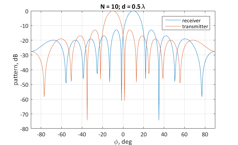
The described feature of the formation of DNs for reception and transmission should always be kept in mind when working with antenna arrays.
Let's play with the radiation pattern
Few highs
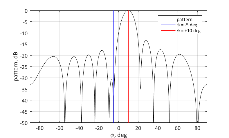
We set the task to form two main maxima of the radiation pattern in the direction: -5 ° and 10 °. To do this, we select the weighted sum of the phasing vectors for the corresponding directions as the weight vector.
$$ display $$ \ textbf {w} = \ beta \ textbf {s} (10 °) + (1- \ beta) \ textbf {s} (- 5 °) $$ display $$
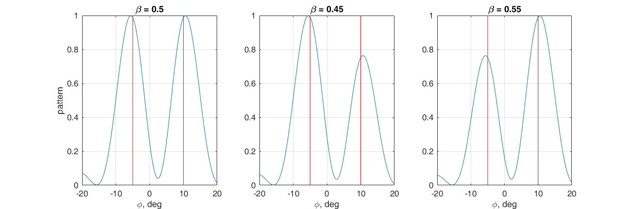 By adjusting the coefficient β, you can adjust the ratio between the main lobes. Here again it is convenient to look at what is happening in the vector space. If β is more than 0.5, then the vector of weight coefficients lies closer to s (10 °), otherwise to s (-5 °). The closer the weight vector is to one of the phasors, the greater is the corresponding scalar product, and hence the magnitude of the corresponding maximum of the DN .
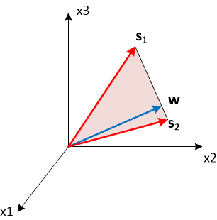
However, it is worth considering that both main petals have a finite width, and if we want to tune in two close directions, then these petals will merge into one, oriented to some middle direction.
One maximum and zero
Now let's try to adjust the maximum radiation pattern to the direction $ inline $ \ phi_1 = 10 ° $ inline $ and simultaneously suppress the signal coming from the direction $ inline $ \ phi_2 = -5 ° $ inline $ . To do this, you need to set a zero for the corresponding angle. You can do this as follows:
$$ display $$ \ textbf {w} = \ textbf {s} _1- \ frac {\ textbf {s} _2 ^ H \ textbf {s} _1} {N} \ textbf {s} _2 $$ display $$
Where $ inline $ \ textbf {s} _1 = \ textbf {s} (10 °) $ inline $ , but $ inline $ \ textbf {s} _2 = \ textbf {s} (- 5 °) $ inline $ .
The geometric meaning of the choice of the weight vector is as follows. We want this vector w to have the maximum projection on $ inline $ \ textbf {s} _1 $ inline $ and at the same time was orthogonal to the vector $ inline $ \ textbf {s} _2 $ inline $ . Vector $ inline $ \ textbf {s} _1 $ inline $ can be represented as two components: a collinear vector $ inline $ \ textbf {s} _2 $ inline $ and orthogonal vector $ inline $ \ textbf {s} _2 $ inline $ . To satisfy the formulation of the problem, it is necessary to choose the second component as a vector of weight coefficients w . You can calculate the collinear component by designing a vector $ inline $ \ textbf {s} _1 $ inline $ to normalized vector $ inline $ \ frac {\ textbf {s} _2} {\ sqrt {N}} $ inline $ using scalar product.
$$ display $$ \ textbf {s} _ {1 ||} = \ frac {\ textbf {s} _2} {\ sqrt {N}} \ frac {\ textbf {s} _2 ^ H \ textbf {s} _1} {\ sqrt {N}} $$ display $$
Accordingly, subtracting from the original phasing vector $ inline $ \ textbf {s} _1 $ inline $ its collinear component, we obtain the desired weight vector.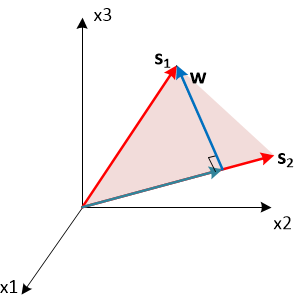
Some additional notes
- Everywhere above, I dropped the question of the normalization of the weight vector, i.e. its length. So, the normalization of the weight vector does not affect the characteristics of the antenna pattern: the direction of the main maxim, the width of the main lobe, etc. It can also be shown that this normalization does not affect the SNR at the output of the spatial processing unit. In this regard, when considering algorithms for spatial signal processing, I usually take a unit normalization of the weight vector, i.e. $ inline $ \ textbf {w} ^ H \ textbf {w} = 1 $ inline $
- The possibilities for the formation of the antenna pattern of the antenna array are determined by the number of elements N. The more elements, the wider the possibilities. The more degrees of freedom in the implementation of spatial weight processing, the more options how to "twist" the weight vector in N-dimensional space.
- In the implementation of the reception of the antenna pattern, the antenna array does not physically exist, and all this exists only in the “imagination” of the computing unit that performs signal processing. This means that at the same time point it is possible to synthesize several days and independently process signals coming from different directions. In the case of transmission, everything is somewhat more complicated, but it is also possible to synthesize several DNs for the transmission of various data streams. This technology in communication systems is called MIMO .
- With the help of the presented matlab code you can play around with NAM yourself.Code
% antenna array settings N = 10; % number of elements d = 0.5; % period of antenna array wLength = 1; % wavelength mode = 'receiver'; % receiver or transmitter % weights of antenna array w = ones(N,1); % w = 0.5 + 0.3*cos(2*pi*((0:N-1)-0.5*(N-1))/N).'; % w = 0.5 - 0.3*cos(2*pi*((0:N-1)-0.5*(N-1))/N).'; % w = exp(2i*pi*d/wLength*sin(10/180*pi)*(0:N-1)).'; % b = 0.5; w = b*exp(2i*pi*d/wLength*sin(+10/180*pi)*(0:N-1)).' + (1-b)*exp(2i*pi*d/wLength*sin(-5/180*pi)*(0:N-1)).'; % b = 0.5; w = b*exp(2i*pi*d/wLength*sin(+3/180*pi)*(0:N-1)).' + (1-b)*exp(2i*pi*d/wLength*sin(-3/180*pi)*(0:N-1)).'; % s1 = exp(2i*pi*d/wLength*sin(10/180*pi)*(0:N-1)).'; % s2 = exp(2i*pi*d/wLength*sin(-5/180*pi)*(0:N-1)).'; % w = s1 - (1/N)*s2*s2'*s1; % w = s1; % normalize weights w = w./sqrt(sum(abs(w).^2)); % set of angle values to calculate pattern angGrid_deg = (-90:0.5:90); % convert degree to radian angGrid = angGrid_deg * pi / 180; % calculate set of steerage vectors for angle grid switch (mode) case 'receiver' s = exp(2i*pi*d/wLength*bsxfun(@times,(0:N-1)',sin(angGrid))); case 'transmitter' s = exp(-2i*pi*d/wLength*bsxfun(@times,(0:N-1)',sin(angGrid))); end % calculate pattern y = (abs(w'*s)).^2; %linear scale plot(angGrid_deg,y/max(y)); grid on; xlim([-90 90]); % log scale % plot(angGrid_deg,10*log10(y/max(y))); % grid on; % xlim([-90 90]);
What tasks can be solved using an adaptive antenna array?
Thanks for attention
Source: https://habr.com/ru/post/449794/
All Articles