Wavelet analysis. The basics

Introduction

The English word wavelet (from French “ondelette”) literally translates as “short (small) wave”. In various translations of foreign articles into Russian there are more terms: “surge”, “wavelet function”, “low wavelength function”, “wave”, etc.

Wavelet transform (VP) is widely used for signal analysis. In addition, it finds a great use in data compression. A VP of a one-dimensional signal is its representation in the form of a generalized series or Fourier integral over a system of basis functions.

p s i_{a b} (t) = f r a c 1 s q r t a p s i l e f t (f r a c t - b a r i g h t)

$\ psi _ {ab} (t) = \ frac {1} {\ sqrt {a}} \ psi \ left (\ frac {t-b} {a} \ right)$ , (one)
')
constructed from the mother (source) wavelet

p s i (t)

$\ psi (t)$ having certain properties due to the operations of shift in time (b) and changes in the time scale (a).

Factor

1 / s q r t a

$1 / \ sqrt {a}$ ensures the independence of the norm of functions (1) on the scaling number (a). For the given values of the parameters a and b function

p s i_{a b} (t)

$\ psi_ {ab} (t)$ and there is a wavelet generated by the mother wavelet

p s i (t)

$\ psi (t)$ .

As an example, we present the “Mexican hat” wavelet in the time and frequency domains:

Wavelet listing for the time domain

from numpy import* import matplotlib.pyplot as plt x= arange(-4,30,0.01) def w(a,b,t): f =(1/a**0.5)*exp(-0.5*((tb)/a)**2)* (((tb)/a)**2-1) return f plt.title(" « »:\n$1/\sqrt{a}*exp(-0,5*t^{2}/a^{2})*(t^{2}-1)$") y=[w(1,0,t) for t in x] plt.plot(x,y,label="$\psi(t)$ a=1,b=12") y=[w(2,12,t) for t in x] plt.plot(x,y,label="$\psi_{ab}(t)$ a=2 b=12") y=[w(4,12,t) for t in x] plt.plot(x,y,label="$\psi_{ab}(t)$ a=4 b=12") plt.legend(loc='best') plt.grid(True) plt.show()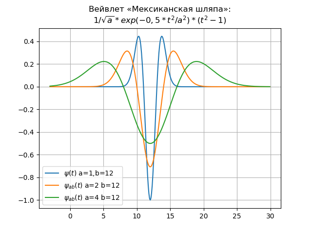

Listing for wavelet spectrum

 from numpy import* from pylab import * from scipy import * import os def w(a,b,t): f =(1/a**0.5)*exp(-0.5*((tb)/a)**2)* (((tb)/a)**2-1) return f x= arange(-4,30,0.2) def plotSpectrum(y,Fs): n = len(y) k = arange(n) T = n/Fs frq = k/T frq = frq[range(int(n/2))] Y = fft(y)/n Y = Y[range(int(n/2))] return Y,frq xlabel('f (Hz)') ylabel('|Y(f)|') Fs=1024.0 y=[w(1,12,t) for t in x] Y,frq=plotSpectrum(y,Fs) plot(frq,abs(Y),label="$\psi(\omega)$ a=1,b=12") y=[w(2,12,t) for t in x] Y,frq=plotSpectrum(y,Fs) plot(frq,abs(Y),label="$\psi_{ab}(\omega)$ a=2 b=12") y=[w(4,12,t) for t in x] Y,frq=plotSpectrum(y,Fs) plot(frq,abs(Y),label="$\psi_{ab}(\omega)$ a=4 b=12") plt.title(" « »   $\omega$") legend(loc='best') grid(True) show()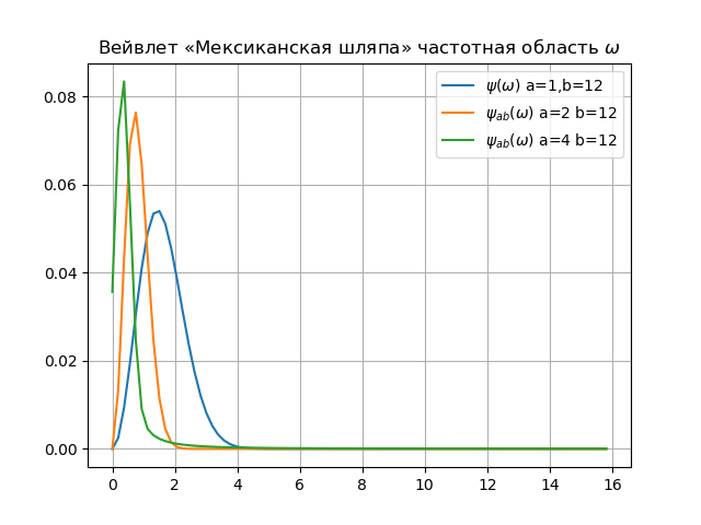

Conclusion:

1. Between the concept of Fourier harmonics and the wavelet scale there is indeed a relationship. The main thing in this relationship is the inverse proportionality of the natural frequency and scale. In addition, by reducing the scale, we increase the bandwidth of the wavelet spectrum.

2. By changing the scale (an increase in a leads to a narrowing of the Fourier spectrum of the function

p s i_{a b} (t)

$\ psi_ {ab} (t)$ ), wavelets are able to detect differences in characteristics at different scales (frequencies), and due to a shift, analyze the properties of the signal at different points throughout the studied interval. Therefore, when analyzing non-stationary signals, due to the locality property of wavelets, they get a significant advantage over the Fourier transform, which gives only global information about the frequencies (scales) of the signal being analyzed, since the system of functions used (complex exponent or sines and cosines) is defined on infinite interval.

3. The above listings, written in a free high-level language, Python allow you to select wavelet functions that meet specified requirements. However, in addition, it is necessary to take into account all the main features of the wavelets.

The main signs of wavelet

Limitations. The square of the norm of the function must be finite:

l e f t | p s i r i g h t |^{2} = i n t_{- i n f t y}^{i n f t y} l e f t | p s i (t) r i g h t |^{2} d t < i n f t y

$\ left \ | \ psi \ right \ | ^ {2} = \ int _ {- \ infty} ^ {\ infty} \ left | \ psi (t) \ right | ^ {2} dt <\ infty$ . (2)

Localization. VP, in contrast to the Fourier transform, uses a localized source function both in time and in frequency. For this it is enough that the following conditions are met:

l e f t | p s i (t) r i g h t | l e q C (1 + l e f t | t r i g h t |)^{- 1 - v a r e p s i l o n}

$\ left | \ psi (t) \ right | \ leq C (1+ \ left | t \ right |) ^ {- 1- \ varepsilon}$ and

l e f t | S_{p s i} (o m e g a) r i g h t | l e q C (1 + l e f t | o m e g a r i g h t |)^{- 1 - v a r e p s i l o n}

$\ left | S _ {\ psi} (\ omega) \ right | \ leq C (1+ \ left | \ omega \ right |) ^ {- 1- \ varepsilon}$ at

v a r e p s i l o n > 0

$\ varepsilon> 0$ , (3)

For example, the delta function

d e l t a (t)

$\ delta (t)$ and the harmonic function does not satisfy the necessary condition for simultaneous localization in the time and frequency domains.

Zero average. The graph of the original function must oscillate (be alternating) around zero on the time axis and have zero area:

i n t_{- i n f t y}^{i n f t y} p s i (t) d t = 0

$\ int _ {- \ infty} ^ {\ infty} \ psi (t) dt = 0$ . (four)

From this condition it becomes clear the choice of the name “wavelet” - a small wave.

Equality zero area function

p s i (t)

$\ psi (t)$ i.e. zero momentum, leads to the fact that the Fourier transform

S_{p s i} (o m e g a)

$S _ {\ psi} (\ omega)$ this function is zero when

o m e g a = 0

$\ omega = 0$ and has the form of a bandpass filter. With different values (a) this will be a set of bandpass filters.

Often, for applications, it is necessary that not only zero, but all the first n moments should be zero:

i n t_{- i n f t y}^{i n f t y} t^{^{n}} p s i (t) d t = 0

$\ int _ {- \ infty} ^ {\ infty} t ^ {^ {n}} \ psi (t) dt = 0$ . (five)

Wavelets of the nth order make it possible to analyze the finer (high-frequency) structure of the signal, suppressing its slowly varying components.

Automaking. A characteristic feature of the EP is its self-similarity. All wavelets of a specific family

p s i_{a b} (t)

$\ psi_ {ab} (t)$ have the same number of oscillations as the mother wavelet

p s i (t)

$\ psi (t)$ , since obtained from it by means of scale transformations (a) and shift (b).

Continuous wavelet transform

Continuous (integral) wavelet transform (NVP or CWT - continuous wavelet transform). We construct the basis

p s i_{a b} (t)

$\ psi_ {ab} (t)$ using continuous scale transformations (a) and transfers (b) of the mother wavelet

p s i (t)

$\ psi (t)$ with arbitrary values of the basic parameters a and b in the formula (1).

Then, by definition, the direct (analysis) and reverse (synthesis) of the CWP (i.e., the CST and CST) of the signal S (t) are written as:

W_{s} (a, b) = (S (t), p s i_{a b} (t)) = f r a c 1 s q r t a i n t_{- i n f t y}^{i n f t y} S (t) p s i l e f t (f r a c t b a r i g h t) d t

$W_ {s} (a, b) = (S (t), \ psi _ {ab} (t)) = \ frac {1} {\ sqrt {a}} \ int _ {- \ infty} ^ {\ infty} S (t) \ psi \ left (\ frac {tb} {a} \ right) dt$ , (6)

S (t) = \ frac {1} {C _ {\ psi}} \ int _ {- \ infty} ^ {\ infty} \ int _ {- \ infty} {{infty} W_ {s} (a, b ) \ psi _ {ab} (t) \ frac {dadb} {a ^ {2}}

$S (t) = \ frac {1} {C _ {\ psi}} \ int _ {- \ infty} ^ {\ infty} \ int _ {- \ infty} {{infty} W_ {s} (a, b ) \ psi _ {ab} (t) \ frac {dadb} {a ^ {2}}$ , (7)

Where

C_{p s i}

$C _ {\ psi}$ - the normalizing factor

C_{p s i} = i n t_{- i n f t y}^{i n f t y} l e f t | p s i (o m e g a) r i g h t |^{2} l e f t | o m e g a r i g h t |^{- 1} d o m e g a < i n f t y

$C _ {\ psi} = \ int _ {- \ infty} ^ {\ infty} \ left | \ psi (\ omega) \ right | ^ {2} \ left | \ omega \ right | ^ {- 1} d \ omega <\ infty$
where: (•, •) is the scalar product of the corresponding factors,

m a t h b f p s i (o m e g a)

$\ mathbf {\ psi (\ omega)}$ - wavelet Fourier transform

p s i (t)

$\ psi (t)$ . For orthonormal wavelets

C_{p s i} = 1

$C _ {\ psi} = 1$ .

From (6) it follows that the wavelet spectrum

W_{s} (b, a)

$W_ {s} (b, a)$ (wavelet spectrum, or time-scale-spectrum - time-scale spectrum), in contrast to the Fourier spectrum (single spectrum) is a function of two arguments: the first argument a (time scale) is similar to the oscillation period, i.e. is inverse to the frequency, and the second b is similar to the signal offset along the time axis.

It should be noted that

W_{s} (b, a_{0})

$W_ {s} (b, a_ {0})$ characterizes the time dependence (with

a = a_{0})

$a = a_ {0})$ whereas dependencies

W_{s} (a, b_{0})

$W_ {s} (a, b_ {0})$ frequency dependence can be assigned (at

b = b_{0}

$b = b_ {0}$ ).

If the signal under study S (t) is a single pulse of duration

t a u_{u}

$\ tau_ {u}$ concentrated in the neighborhood

t = t_{0}

$t = t_ {0}$ then its wavelet spectrum will have the greatest value in the vicinity of the point with coordinates

a = t a u_{u}, b = t_{0}

$a = \ tau_ {u}, b = t_ {0}$ .

Ways of representation (visualization)

W_{s} (b, a)

$W_ {s} (b, a)$ may be different. Spectrum

W_{s} (b, a)

$W_ {s} (b, a)$ is a surface in three-dimensional space. However, instead of the image of the surface, they often represent its projection on the ab plane with iso-levels (or figures of different colors), which allow tracing the change in the intensity of the amplitudes of the EPs at different scales (a) and in time (b).

In addition, they depict pictures of local extremum lines of these surfaces, the so-called skeleton, which reveals the structure of the signal being analyzed.

The continuous wavelet transform in determining the wavelet spectrum based on the maternal wavelet is a “Mexican hat”.

Other maternal wavelets used for NVP are also used:

Continuous VP has found wide application in signal processing. In particular, wavelet analysis (VA) provides unique opportunities to recognize local and “subtle” features of signals (functions), which is important in many areas of radio engineering, communications, radio electronics, geophysics, and other branches of science and technology. Consider this possibility in some of the simplest examples.

Harmonic oscillation

The signal is:

s (t) = A s i n (o m e g a t - p h i)

$s (t) = Asin (\ omega t- \ phi)$

Where:

A = 1 V, o m e g a = f r a c 2 p i T = f r a c 2 p i 50, p s i = 0

$A = 1 V, \ omega = \ frac {2 \ pi} {T} = \ frac {2 \ pi} {50}, \ psi = 0$

Wavelet function:

M H A T (t) := f r a c d^{2} d t^{2} e x p (- t^{2} / 2)

$MHAT (t): = \ frac {d ^ {2}} {dt ^ {2}} exp (-t ^ {2} / 2)$ ,

Wavelets:

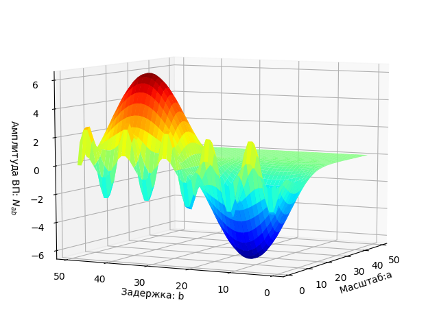
p s i (a, b, t) = f r a c 1 s q r t a M H A T l e f t (f r a c t - b a r i g h t)

$\ psi (a, b, t) = \ frac {1} {\ sqrt {a}} MHAT \ left (\ frac {t-b} {a} \ right)$ ,

Wavelet spectrum: N: = 256, a: = 1..30, b: = 0..50,

W (a, b) := i n t_{- N}^{N} p s i (a, b, t) s (t) d t, N_{a b} := W (a, b) .

$W (a, b): = \ int _ {- N} ^ {N} \ psi (a, b, t) s (t) dt, N_ {ab}: = W (a, b).$ .

Program listing

 from scipy.integrate import quad from numpy import* import matplotlib.pyplot as plt from mpl_toolkits.mplot3d import Axes3D from matplotlib import cm N=256 T=50 def S(t): return sin(2*pi*t/T) plt.figure() plt.title('  ', size=12) y=[S(t) for t in arange(0,100,1)] x=[t for t in arange(0,100,1)] plt.plot(x,y) plt.grid() def w(a,b): f = lambda t :(1/a**0.5)*exp(-0.5*((tb)/a)**2)* (((tb)/a)**2-1)*S(t) r= quad(f, -N, N) return round(r[0],3) x = arange(1,50,1) y = arange(1,50,1) z = array([w(i,j) for j in y for i in x]) X, Y = meshgrid(x, y) Z = z.reshape(49,49) fig = plt.figure("- :  ") ax = Axes3D(fig) ax.plot_surface(X, Y, Z, rstride=1, cstride=1, cmap=cm.jet) ax.set_xlabel(' :a') ax.set_ylabel(': b') ax.set_zlabel(' : $ N_{ab}$') plt.figure("2D-  z = w (a,b)") plt.title(' ab    ', size=12) plt.contourf(X, Y, Z,100) plt.show()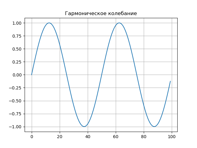

Signal graph.

Graph of the two-parameter spectrum

N_{a b} = W (a b)

$N_ {ab} = W (ab)$ displayed as a surface in three-dimensional space.

It should be noted that the W (a, b) section for the time scale

a = a_{0}

$a = a_ {0}$ characterizes the original oscillation s (t). In this case, its amplitude is maximum at

a_{0} : 1 / o m e g a

$a_ {0}: 1 / \ omega$ . Dependencies

W (a_{0}, b_{0})

$W (a_ {0}, b_ {0})$ the current spectrum of oscillation can be assigned to

b = b_{0}

$b = b_ {0}$ .

The sum of two harmonic oscillations.

The signal is:

s (t) := A_{1} s i n (o m e g a_{1} t) + A_{2} s i n (o m e g a_{2} t)

$s (t): = A_ {1} sin (\ omega _ {1} t) + A_ {2} sin (\ omega _ {2} t)$

Where:

A_{1} = A_{2} = 1 V, o m e g a_{1} = f r a c 2 p i T_{1}, o m e g a_{2} = f r a c 2 p i T_{2}, T_{1} = 50 s, T_{2} = 10 s

$A_ {1} = A_ {2} = 1V, \ omega_ {1} = \ frac {2 \ pi} {T_ {1}}, \ omega_ {2} = \ frac {2 \ pi} {T_ {2 }}, T_ {1} = 50s, T_ {2} = 10s$ .

M H A T (t) := f r a c d^{2} d t^{2} l e f t [e^{- t^{2 / 2}} r i g h t]

$MHAT (t): = \ frac {d ^ {2}} {dt ^ {2}} \ left [e ^ {- t ^ {2/2}} \ right]$ , N: = 256,

p s i (a, b, t) := M H A T l e f t (f r a c t b a r i g h t), W (a, b) := i n t_{- N}^{N} p s i (a, b, t) f (t) d t

$\ psi (a, b, t): = MHAT \ left (\ frac {tb} {a} \ right), W (a, b): = \ int _ {- N} ^ {N} \ psi (a , b, t) f (t) dt$ , a: = 1 ... 30, b: = 0 ... 50,

N_{a b} := W (a, b)

$N_ {ab}: = W (a, b)$ .

Program listing

 from scipy.integrate import quad from numpy import* import matplotlib.pyplot as plt from mpl_toolkits.mplot3d import Axes3D from matplotlib import cm N=256 def S(t): return sin(2*pi*t/10)+sin(2*pi*t/50) plt.figure('    ') plt.title('    ', size=12) y=[S(t) for t in arange(0,250,1)] x=[t for t in arange(0,250,1)] plt.plot(x,y) plt.grid() def w(a,b): f = lambda t :(1/a**0.5)*exp(-0.5*((tb)/a)**2)* (((tb)/a)**2-1)*S(t) r= quad(f, -N, N) return round(r[0],3) x = arange(1,50,1) y = arange(1,50,1) z = array([w(i,j) for j in y for i in x]) X, Y = meshgrid(x, y) Z = z.reshape(49, 49) fig = plt.figure("-:2-  ") ax = Axes3D(fig) ax.plot_surface(X, Y, Z, rstride=1, cstride=1, cmap=cm.jet) ax.set_xlabel(' :a') ax.set_ylabel(': b') ax.set_zlabel(' : $ N_{ab}$') plt.figure("2D-  z = w (a,b)") plt.title(' ab    ', size=12) plt.contourf(X, Y, Z, 100) plt.figure() q=[w(2,i) for i in y] p=[i for i in y] plt.plot(p,q,label='w(2,b)') q=[w(15,i) for i in y] plt.plot(p,q,label='w(15,b)') q=[w(30,i) for i in y] plt.plot(p,q,label='w(30,b)') plt.legend(loc='best') plt.grid(True) plt.figure() q=[w(i,13) for i in x] p=[i for i in x] plt.plot(p,q,label='w(a,13)') q=[w(i,17) for i in x] plt.plot(p,q,label='w(a,17)') plt.legend(loc='best') plt.grid(True) plt.show()

Signal graph.

The graph of the two-parameter spectrum W (a, b) is plotted as a surface in three-dimensional space.

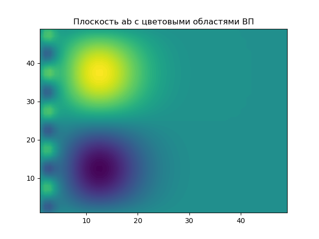
The plane of the parameters a, b on which the results of the EP are highlighted with colored areas.

The graph shows the "cross section" of the wavelet spectrum for two values of the parameter a. With a relatively small time scale parameter a, with

a_{1} = 2 (a_{1} : 1 / o m e g a_{2})

$a_ {1} = 2 (a_ {1}: 1 / \ omega_ {2})$ , the cross section of the spectrum carries information only about the high-frequency component of the signal, filtering (suppressing) its low-frequency component.

As a grows, the base function stretches.

p s i (f r a c t - b a)

$\ psi (\ frac {t-b} {a})$ , therefore, the narrowing of its spectrum, and the narrowing of the frequency bandwidth of the “window”. As a result,

a_{2} = 15 (a_{2} : 1 / o m e g a_{1})

$a_ {2} = 15 (a_ {2}: 1 / \ omega_ {1})$ The cross section of the spectrum is only a low frequency component of the signal.

With a further increase in a, the window band is still reduced and the level of this low-frequency component decreases to a constant component (with a> 25) equal to zero for the analyzed signal.

The graph shows the cross section of the wavelet spectrum W (a, b), characterizing
current signal spectrum at

b_{1} = 13

$b_ {1} = 13$ and

b_{2} = 17

$b_ {2} = 17$ . The spectrum of the considered signal, in contrast to the harmonic signal, contains a high-frequency component in the region of small values of the time scale a (a: 1..3), which corresponds to the second component of the signal

A_{2} s i n (o m e g a_{2} t)

$A_ {2} sin (\ omega_ {2} t)$ .

Rectangular impulse.

U := 5, t_{0} := 20, t a u := $ 6

$U: = 5, t_ {0}: = 20, \ tau: = $ 6$

s (t) := b e g i n v m a t r i x U, i f t_{0} l e q t l e q t_{0} + t a u 0, o t h e r w i s e e n d v m a t r i x

$s (t): = \ begin {vmatrix} U, if t_ {0} \ leq t \ leq t_ {0} + \ tau \\ 0, otherwise \ end {vmatrix}$

M H A T (t) := f r a c d^{2} d t^{2} e x p l e f t (f r a c - t^{2} 2 r i g h t)

$MHAT (t): = \ frac {d ^ {2}} {dt ^ {2}} exp \ left (\ frac {-t ^ {2}} {2} \ right)$

N := 128, p s i (a, b, t) := M H A T l e f t (f r a c t b a r i g h t), W (a, b) := i n t_{- N}^{N} p s i (a, b, t) f (t) d t

$N: = 128, \ psi (a, b, t): = MHAT \ left (\ frac {tb} {a} \ right), W (a, b): = \ int _ {- N} ^ {N } \ psi (a, b, t) f (t) dt$

a := 1..50, b := 0..100, N_{b a} := W (a, b)

$a: = 1..50, b: = 0..100, N_ {ba}: = W (a, b)$

Program listing

 from scipy.integrate import quad from numpy import* import matplotlib.pyplot as plt from mpl_toolkits.mplot3d import Axes3D from matplotlib import cm N=256 def S(t): U=5;t0=20;tau=60 if t0<=t<=t0+tau: return U else: return 0 plt.figure() plt.title(' ', size=12) y=[S(t) for t in arange(0,120,1)] x=[t for t in arange(0,120,1)] plt.plot(x,y) plt.grid() def w(a,b): f = lambda t :(1/a**0.5)*exp(-0.5*((tb)/a)**2)* (((tb)/a)**2-1)*S(t) r= quad(f, -N, N) return round(r[0],3) x = arange(1,100,1) y = arange(1,100,1) z = array([w(i,j) for j in y for i in x]) X, Y = meshgrid(x, y) Z = z.reshape(99, 99) fig = plt.figure("3D-  ") ax = Axes3D(fig) ax.plot_surface(X, Y, Z, rstride=1, cstride=1, cmap=cm.jet) ax.set_xlabel(' :a') ax.set_ylabel(': b') ax.set_zlabel(' : $ N_{ab}$') plt.figure("2D-  z = w (a,b)") plt.title(' ab    ', size=12) plt.contourf(X, Y, Z,100) plt.show()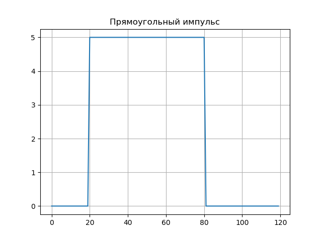

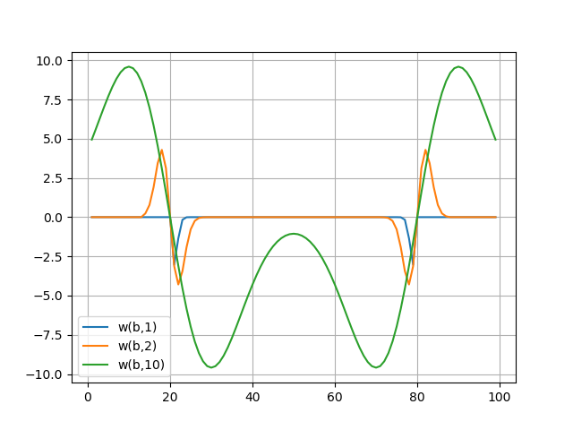
The wavelet spectra are shown in the graphs, the wavelet spectrum well conveys the subtle features of the signal - its jumps in the samples b = 20 and b = 80 (for a: 1..10).

findings

This publication is educational in nature, it contains basic information about wavelet analysis in general, and simple examples of the freely-distributed high-level programming language Python show the features of continuous wavelet analysis with extensive 3D and 2D visualization.

PS The author does not detract from the unconditional advantages of wavelet analysis using Matlab both in terms of the number of wavelets and in speed. But in Python there is still much room for development; it is scipy.signal and PyWavelets.

Source: https://habr.com/ru/post/449646/

All Articles

Wavelet analysis. The basics

Introduction

The main signs of wavelet

Continuous wavelet transform

The continuous wavelet transform in determining the wavelet spectrum based on the maternal wavelet is a “Mexican hat”.

findings

More articles: