New Frontiers in Physics
Hello, dear reader! I present to your attention a translation from English of the article "Physics, The Next Frontier" by Chris Hecker.
I, a novice Java developer, faced with the fact that materials on the creation of a physical in-game engine are presented only in English, which is why this article was translated. There will be three more articles in the series; I will post them as soon as they are ready. Enjoy reading!
There is no doubt that every year the in-game graphics become more realistic. Already today everyone creates (or at least shows screenshots) 3D worlds with texture maps, and when enough hardworking people get together to work on one project, each developer can draw billions of polygons of realistic textures and shadows per second. Technically speaking, what remains to be done to create a game at a high level? Will every developer with a copy of the book “Learn to Use 3D Hardware in 21 Days” be able to create a truly impressive game?
Far from it. High-end developers will continue to raise the bar in a variety of different technologies (such as GUI complexity, artificial intelligence, and networking). Of course, all this is very important, we cannot even seriously discuss any of them without specifying details. Nevertheless, there is one applicable to all technology, which, in my opinion, will be the decisive factor in the near future: physics.
')
Consider the following example: do you remember these huge rotating gears in one of the early levels of Duke Nukem 3D?

Figure 1. Screenshot of the Duke Nukem 3D game
Just imagine that their rotation would be described not by a looping animation, but by a real physics engine. Suddenly, the gears become something more than a game decoration, just as one of them deviates from a given angle, and rolls down the corridor behind you, as in Indiana-Jones films. Or imagine that after a shot at the gear of a rocket launcher, it will roll down the corridor and crush your friend who has crept up behind you to kill you! Physical engines make such situations real.
Physical simulation is what makes the game world whole: thanks to it, “here” is exactly here, if you know what I mean. Any magic in the graphics in the world will not allow the player to immerse himself in the gameplay, if he interpeners with another player, or into the walls of the level, or if the mass and moment of mass will not be felt. Animators at Disney discovered that this mass sensation is what separates good animation from bad. According to the epic book “Disney Animation: The Illusion of Life” by Frank Thomas and Ollie Johnston, animators of Disney, even just hanging a poster in a studio, have to ask themselves the question all the time: “Is there mass in their plotting, depth and balance? ?
But today almost every game has a physics engine, right? Undoubtedly, this is exactly what keeps your car from falling off the edge of the game world, thanks to it your characters do not fly off into space when they jump, and this throws your boat to the side when a rocket explodes nearby. However, most of the physics engines in modern games are rather weak. They only cope with the task of keeping the car from falling off the edge of the world, but their capabilities are not enough to take the game to a new level - where the wreckage of a crashed car can explode right on the track, causing the walls and other cars to roll.
Other physical effects that are often ignored include: from simple twisting effects as a result of striking a tangent, to the point that the characters in the game will keep their balance and move, unlike statically animated ones. I believe that many developers ignore these possibilities, because they do not understand the math, describing physics, or were too busy creating texture maps to learn it. The onslaught of 3D hardware will take care of the latter, and I begin a new series of articles. The first article will take care of the formalities. By the end of our cycle, you yourself will be able to create a physical engine that will cause the players a sense of complete immersion in the gameplay, thanks to incredible realism, or - entertaining, but persistent surrealism.
A warning! Physics = mathematics, in order to complete an interesting project, you will have to use both. Before it scares you away, let me say that mathematics that describes physics is not only elegant and beautiful, it also has an applied character. That is, it is not abstract mathematics for mathematics. Every equation we use has a real physical meaning. We create equations from a physical model, and instead, the equations tell us how the model behaves in time.
Physics is a wide scientific field. We are actually interested in its small section called “dynamics”, or rather, “dynamics of solids”. Dynamics can be defined in terms of a related section — kinematics (the theory of motion in time). Kinematics does not sharpen its focus on what causes movement or how the bodies ended up where they are, it simply describes movement. Dynamics, on the contrary, describes the forces and masses that contribute to the values from the kinematics vary with time. How far the ball for baseball will fly, if the flight time is 10 seconds, and its initial speed is 50 kilometers / hour, and the trajectory - a straight line - is a problem of kinematics; how far a baseball ball flies into the gravitational field of the earth, if I hit it with a bat, this is a dynamic problem.
The part of the dynamics that describes solids is related to the constraints that we add to simulated objects. The shape of a solid body does not change in the course of the simulation - the body is more wooden or metallic than jelly-like. We can create articulated figures, for example, a man, by constructing each part of a figure from a solid body and creating bundles between them, but we will not rely on bones bending under the force of force or similar effects. This will allow us to simplify our equations without losing the quality of the interesting dynamic behavior of bodies.
Even though we consider such a small part of the dynamics, the dynamics of a rigid body will require a series of articles to explain the essence. We will begin our journey by learning the basics of computer programming to describe the motion of a flat rigid body under the action of forces. I persistently repeat “computer programming,” since, in addition to the equations we write for kinematics and dynamics, we will also learn how to solve these equations using floating-point calculations, which is vital for every programmer to know. I say “flat solid” because we will only deal with the two-dimensional world for the next article and beyond. Principles - and in fact more than just equations - may be shifted to the three-dimensional world as well, but definitely everything is much simpler in a two-dimensional one, so we will study there until we feel confident to enter the three-dimensional space. In future articles we will learn to describe the effect of rotation, the processing of body contacts, and, of course, how to do all this in a three-dimensional world. Well, enough words! Let's start!
This may come as a surprise to you, but you really can't move an object just by pushing it. I know you think I'm wrong, proving me otherwise by throwing this magazine in the trash for writing such nonsense, but it's true! Only putting pressure on a magazine will never directly affect its position in space. In fact, exerting pressure does not even directly affect its speed. What pressure really affects is the acceleration of the journal, and in fact it is one of the most important conclusions in the history of science.
In order to use this fact in order to do something interesting, we first need to talk about the relationship of body position with speed and acceleration. In reality, all these values are very closely related (as you probably know): speed is an indicator of a change in body coordinates with time, and acceleration is an indicator of a change in speed. The primary tool for studying changes in these quantities over time is differential calculus. If you understand this, then we go further. I guess you are good at math. We will use only simple scalar and vector calculations (derivatives and integrals), but it will not be superfluous if you are familiar with mathematics in general. For reference: my favorite book on calculations is Calculus with Analytic Geometry by Thomas and Finney.
Coordinate, speed and acceleration are the magnitudes of the kinematics discussed in this article. The location of a solid body in a two-dimensional world is, obviously, a pair of X and Y coordinates, which denote the space coordinates of some given point of the body. The derivative for the coordinate vector is the velocity vector, and it shows us in which direction the point moves (and the body, if we ignore the rotation, which is happening now) and how fast it moves. Vector calculus is simply the scalar calculus of each element of a vector, so the derivative of the X coordinate is the velocity of the body in X, and so on. We introduce the following notation. Let the coordinate of the body be the vector r, and the speed be the vector v or vector r with a stroke. We get the equation:
Equation 1
If we differentiate the velocity vector over time, it will show how the coordinate vector changes with time. Acceleration is determined by analogy. This is the first derivative of the velocity or the second derivative of the coordinate vector:
Equation 2
The integral of the acceleration will give us the speed, and by integrating the acceleration twice, we get the coordinate.
These relationships in kinematics show that we can find the acceleration of an object, we can integrate it over time to get speed and coordinate. As we will see later, we will turn to integration many times in our code for simulation and will calculate a new position for our solid body for each frame. Cheers animation!
Here is a simple example for a one-dimensional world, which we can analytically integrate. We agree that we want to find a change in the coordinates from the end of the last frame to the current frame to draw the current position. Then we say that the acceleration of our solid body was equal to 5 arbitrary units / second ^ 2. We will use the time elapsed since the end of the last frame as the variable t (in the integration element dt).
Equation 3
The above equations show that speed is a function of the time since the last frame. We found an integration constant, C, which is equal to the initial velocity at the beginning of the integration period (at t = 0).
Equation 4
Now we will integrate our velocity equation to find the coordinate (again, do not forget about the integration constant):
Equation 5
Based on Equation 5, we can find the current position only by the given acceleration, if we know the initial coordinate and speed (which we take from the last frame) and the elapsed time. The input variable is time, and the value of the function is the current position. We will also specify the time in Equation 4 to calculate the final rate so that we can use this as the initial condition for the next frame.
Now we have the realization that it is necessary to set the acceleration correctly in order to integrate the kinematic equations to get the animation. The output of the speakers on the scene. Remember how I said that by pushing on something, you directly affect only the acceleration of the body? Well, “exerting pressure” is just a euphemism for the phrase “apply force” - one of two key variables in dynamics - and now we can turn to Newton to find out how forces affect acceleration. Newton's second law connects the force F with the derivative of the mass — the second value of the dynamics — multiplied by the speed. The product of mass and velocity is called the “body momentum”, denoted by p:
Equation 6
Mass is a constant for the speeds with which we are currently working, it follows from the derivative in Equation 6, and we obtained the well-known equation F = ma (although I am sure that Newton initially determined the force through the derivative of momentum).
If we dealt only with material points, Equation 6 is what we need in dynamics. For a given force of a given material point, the acceleration is found by dividing the force by the mass. This gives us an acceleration that will help solve the equation of motion from the example above. Nevertheless, we are dealing with solid bodies with a mass distributed over a certain area (volume, when it comes to the three-dimensional world), so we need to work more.
First, consider a solid body, as a set of point masses. We define the total impulse, pT, for a solid, as the sum of the impulses of all the points that make up the body (I use upper indexing, because I want to show more clearly which quantities belong to these points):
Equation 7
We can significantly simplify the analysis of the dynamics of a solid body by introducing the concept of the center of mass (CM). The vector directed to the center of mass is the linear sum of the vectors directed from all points of the mass of a solid body divided by the mass of the whole body, M:
Equation 8
Using the definition of the center of mass, we can simplify Equation 7 by multiplying both sides of Equation 8 by M, differentiating them, and then substituting the result into Equation 7:
Equation 9
The right side of Equation 9 is the total momentum by definition in Equation 7. Now look at the left side of the equation: this is the velocity at the center of mass multiplied by the mass of the whole body. Move the right side to the left and get:
Equation 10
From Equation 10 it follows that the linear impulse is equal to the total mass multiplied by the speed directed from the center of mass, therefore there is no need to sum up in Equation 7 in order to find the impulse if we know the body mass and the direction of the velocity vector of the center of mass. Further, all final results of the calculations are finding the integrals for the whole body, but the center of mass exists and greatly simplifies finding the total momentum from Equation 10, therefore we can not survive - to find a linear momentum we can consider the body as a material point with given speed and mass.
By analogy, the total force is a derivative of the total momentum, so the concept of the center of mass can also be used to simplify the force equation:
Equation 11
In short, it follows from Equation 11 that we can consider all forces interacting with a solid body, as if their sum vector had an effect on the center of mass point, which contains the mass of the whole body. We divide the force (read gravity) by M in order to find the acceleration of the center of mass, and then we integrate the acceleration over time in order to get the speed and the coordinate of the body. Because we ignore the effects of rotation until the next article; we already have all the equations that we need to describe the dynamics of a rigid body. Note that Equation 11 does not contain information on where the forces applied to the body are directed. This will come up when we deal with a linear impulse and center of mass, and we simply apply forces to CM to find the acceleration of the center of mass. When we calculate the rotation of the body under the action of these forces in the next article, we will see how the coordinate of the application of force is used.
At this stage, we can consider another example of analytical integration using Equation 11 to find the acceleration of the center of mass instead of an arbitrarily chosen quantity = 5. However, we are faced with a serious problem, since analytical integration usually has no practical value because it is too complicated, so we will stop at the so-called numerical integration of ordinary differential equations (ODE). Wow, now it sounds like real math! Once you learn this, it’s time to raise the bar. Fortunately, the numerical integration of an ODE is not as difficult as it may seem at first glance! In order to understand what it means, let's move from words to deeds!
So, a differential equation is an equation that contains derivatives of dependent variables in addition to the function itself, independent variables and parameters. This is wordy, but here is an example for a time-varying force in a one-dimensional world: F = 2t, F is a dependent quantity, and t is an independent one. The value of F is determined only by F. Let the equation of force depend only on the speed of our body. The force of air resistance increases with increasing speed of the aircraft. Let us return to the example in the one-dimensional world, what if F = -v means that the friction force slows down our body in proportion to the speed? We have a problem, because we solve the equation as follows: F = ma = -v and, dividing by m, we get (remember that acceleration is a derivative of speed):
Equation 12
This differential equation, (the equation of speed contains the derivative of speed in Equation 12) is called an ordinary differential equation, because it contains only ordinary derivatives of dependent quantities (as opposed to partial derivatives, which make up partial differential equations [PDI], which we will not talk about ).
We now turn to the next part of our phrase: integration. How did we integrate dv / dt to find v under the conditions of this equation?
This will seem incredible, but almost every equation in physics is differential, so the ODEs have been well studied. Differential equations are so often found in physics, because often the rate of change of a quantity value depends on the quantity itself. For example, we have already noted that braking (the magnitude of the change in speed), including the speed of air resistance, depends on the speed. Other examples from physics are: cooling (the rate of heat loss depends on the current temperature) and radioactive decay (the rate of decay depends on how much radioactive material is present).
The final word in our phrase is numerical - our salvation. I say this because the theory of analytic integration of differential equations, even the simplest, is huge and rather complicated. Although, ironically, the integration of ODE by computer numerical methods is in fact relatively easy to understand. Next, I will describe a simple numerical integrator based on the Euler method, and modify it in the next article.
Almost all numerical integrators, but no other as explicitly as the Euler method, are based simply on the old definition of computation through the first derivative of an oblique: dy / dx determines the slope of y depending on x. For example, if we have a linear equation y = 5x, then dy / dx = 5 means that the slope is a constant equal to 5 for any x, and, as we can assume, it is direct. A slightly more difficult example is the parabola y = x2. In this case, dy / dx = 2x, and this is a function, to determine the new inclined for each x coordinate. I depicted y = x2 in Figure 2:
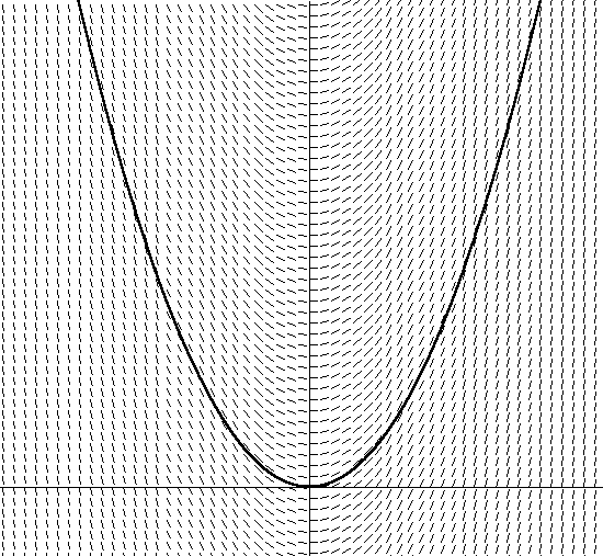
Figure 2. y = x2
In addition to this, I also depicted with the hatching the direction of the vector oblique, solving the equation dy / dx = 2x + C for all x. Note that the angle of the oblique vector is equal to the tangent of the angle of the tangent at the given point. Note also that there are many different parabolas that satisfy the angle of the set of tangents that differ only in the y-axis shift. Each of these parabolas is obtained by using different integration constants, which are contained in the equation dy / dx = 2x + C. The parabola I depicted has an integration constant of 0. If I choose another constant, for example, 1, I get the equation y = 2x + 1. This means that there is a similar parabola with a shift of 1 unit up the y axis.
Now think about the fact that if you do not know the field of vectors in Figure 2, defined by a parabola, then just sit in a puddle. So, if you want to solve the tangent equation, you just need to follow the direction of the vector at each point, changing direction to match the change in direction of the vector field. You will be surprised that after some time, you will see that you are moving along a parabolic trajectory (or a parabola section), depending on where you started. Without realizing it, you have integrated the vector field equation. You found a specific parabola (depending on where you started, or on the initial conditions), using only the derivative equation (calculating dy / dx as you move in the vector field).
Doing the same for a real differential equation is also easy. For a differential equation of the type dy / dx = f (x, y), finding the derivative dy / dx as tangent to f (x, y) describes the angle of inclination of the tangent for each coordinate on the x, y graph. If you depict a graph of a vector field given by dy / dx = f (x, y), you can follow this by analogy with a parabola, by finding the derivative at each point and following in this direction. Figure 2 shows the vector field for Equation 12, our air resistance equation, with speed along the vertical axis and time along the horizontal (I arbitrarily chose m = 1 for this graph).
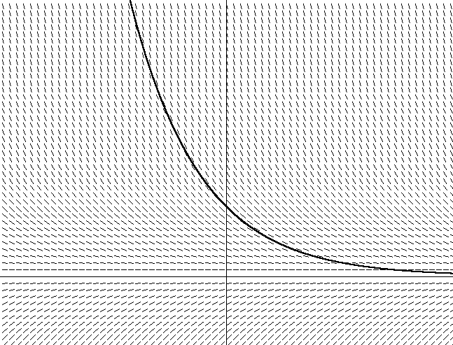
Figure 3. dv / dt = -v / m
It also shows one of the many possible curves. It can be noted that if you select the starting position in the graph (which depends on the initial velocity in the equation), over time the speed will tend to zero, because the friction force slows down the body. You can also see how the decrease in the value of speed depends on the current value of speed - the faster you move, the faster it decreases. This becomes apparent when the same thing follows from Equation 12.
Numerical integration is similar to what we did on the graph. The Euler algorithm for numerical integration simply follows the vector field in accordance with the initial position by finding the derivative of the equation (-v / m for our example with friction force) to determine the slope at the current point, and then simply advances step by step in time, depending on unchanged value of h, along the line of inclination. Then a new position is calculated to determine the new slope after a certain time period:
Or more precisely for our air resistance equation:
Obviously, the Euler method gives a small error with each time step, since the real velocity vector (and therefore the solution curve) bends with a deviation in each point, and the Euler algorithm slightly deviates from the angle of inclination. But if the time step, h are rather small values, the error tends to zero. We will discuss this in more detail in the future.
This is all you need to know about numerical integration by the Euler method. You may ask how we are going to integrate the speed to get the coordinate. We simply use again the Euler method for integrating dr / dt = v, in the same way as integrating dv / dt = a, by analogy. We get two related differential equations (another our victory):
This gives us an alternative algorithm for calculating the coordinates after the action of any arbitrarily applied force on our object (which may depend on speed, as we have seen, or time, or even the position of our body and other bodies, or on everything at once!). For the Euler method, it doesn’t matter what the applied force looks like, since you can calculate it at any time. Euler is interested in the magnitude of the effect of force on mass, as it is inclined, and that’s all.
I ran out of space, so I don’t have the opportunity to provide links. Next time I will recommend various wonderful books, and we will figure out how to calculate the rotation of solids.
And although his body is not as solid as we would like, Chris Hecker has a dynamic personality. If you apply force, he will respond to e-mail checker@bix.com.
Translator's notes: here is a play on words, the topic of the article and its content are played up.
PS The author of the translation expresses a special thanks to the users berez and MarazmDed for their editing of the translation. Thank!
I, a novice Java developer, faced with the fact that materials on the creation of a physical in-game engine are presented only in English, which is why this article was translated. There will be three more articles in the series; I will post them as soon as they are ready. Enjoy reading!
New Frontiers in Physics
There is no doubt that every year the in-game graphics become more realistic. Already today everyone creates (or at least shows screenshots) 3D worlds with texture maps, and when enough hardworking people get together to work on one project, each developer can draw billions of polygons of realistic textures and shadows per second. Technically speaking, what remains to be done to create a game at a high level? Will every developer with a copy of the book “Learn to Use 3D Hardware in 21 Days” be able to create a truly impressive game?
Far from it. High-end developers will continue to raise the bar in a variety of different technologies (such as GUI complexity, artificial intelligence, and networking). Of course, all this is very important, we cannot even seriously discuss any of them without specifying details. Nevertheless, there is one applicable to all technology, which, in my opinion, will be the decisive factor in the near future: physics.
')
Consider the following example: do you remember these huge rotating gears in one of the early levels of Duke Nukem 3D?
Figure 1. Screenshot of the Duke Nukem 3D game
Just imagine that their rotation would be described not by a looping animation, but by a real physics engine. Suddenly, the gears become something more than a game decoration, just as one of them deviates from a given angle, and rolls down the corridor behind you, as in Indiana-Jones films. Or imagine that after a shot at the gear of a rocket launcher, it will roll down the corridor and crush your friend who has crept up behind you to kill you! Physical engines make such situations real.
Physical simulation is what makes the game world whole: thanks to it, “here” is exactly here, if you know what I mean. Any magic in the graphics in the world will not allow the player to immerse himself in the gameplay, if he interpeners with another player, or into the walls of the level, or if the mass and moment of mass will not be felt. Animators at Disney discovered that this mass sensation is what separates good animation from bad. According to the epic book “Disney Animation: The Illusion of Life” by Frank Thomas and Ollie Johnston, animators of Disney, even just hanging a poster in a studio, have to ask themselves the question all the time: “Is there mass in their plotting, depth and balance? ?
But today almost every game has a physics engine, right? Undoubtedly, this is exactly what keeps your car from falling off the edge of the game world, thanks to it your characters do not fly off into space when they jump, and this throws your boat to the side when a rocket explodes nearby. However, most of the physics engines in modern games are rather weak. They only cope with the task of keeping the car from falling off the edge of the world, but their capabilities are not enough to take the game to a new level - where the wreckage of a crashed car can explode right on the track, causing the walls and other cars to roll.
Other physical effects that are often ignored include: from simple twisting effects as a result of striking a tangent, to the point that the characters in the game will keep their balance and move, unlike statically animated ones. I believe that many developers ignore these possibilities, because they do not understand the math, describing physics, or were too busy creating texture maps to learn it. The onslaught of 3D hardware will take care of the latter, and I begin a new series of articles. The first article will take care of the formalities. By the end of our cycle, you yourself will be able to create a physical engine that will cause the players a sense of complete immersion in the gameplay, thanks to incredible realism, or - entertaining, but persistent surrealism.
A warning! Physics = mathematics, in order to complete an interesting project, you will have to use both. Before it scares you away, let me say that mathematics that describes physics is not only elegant and beautiful, it also has an applied character. That is, it is not abstract mathematics for mathematics. Every equation we use has a real physical meaning. We create equations from a physical model, and instead, the equations tell us how the model behaves in time.
Big business
Physics is a wide scientific field. We are actually interested in its small section called “dynamics”, or rather, “dynamics of solids”. Dynamics can be defined in terms of a related section — kinematics (the theory of motion in time). Kinematics does not sharpen its focus on what causes movement or how the bodies ended up where they are, it simply describes movement. Dynamics, on the contrary, describes the forces and masses that contribute to the values from the kinematics vary with time. How far the ball for baseball will fly, if the flight time is 10 seconds, and its initial speed is 50 kilometers / hour, and the trajectory - a straight line - is a problem of kinematics; how far a baseball ball flies into the gravitational field of the earth, if I hit it with a bat, this is a dynamic problem.
The part of the dynamics that describes solids is related to the constraints that we add to simulated objects. The shape of a solid body does not change in the course of the simulation - the body is more wooden or metallic than jelly-like. We can create articulated figures, for example, a man, by constructing each part of a figure from a solid body and creating bundles between them, but we will not rely on bones bending under the force of force or similar effects. This will allow us to simplify our equations without losing the quality of the interesting dynamic behavior of bodies.
Even though we consider such a small part of the dynamics, the dynamics of a rigid body will require a series of articles to explain the essence. We will begin our journey by learning the basics of computer programming to describe the motion of a flat rigid body under the action of forces. I persistently repeat “computer programming,” since, in addition to the equations we write for kinematics and dynamics, we will also learn how to solve these equations using floating-point calculations, which is vital for every programmer to know. I say “flat solid” because we will only deal with the two-dimensional world for the next article and beyond. Principles - and in fact more than just equations - may be shifted to the three-dimensional world as well, but definitely everything is much simpler in a two-dimensional one, so we will study there until we feel confident to enter the three-dimensional space. In future articles we will learn to describe the effect of rotation, the processing of body contacts, and, of course, how to do all this in a three-dimensional world. Well, enough words! Let's start!
Work with derivative
This may come as a surprise to you, but you really can't move an object just by pushing it. I know you think I'm wrong, proving me otherwise by throwing this magazine in the trash for writing such nonsense, but it's true! Only putting pressure on a magazine will never directly affect its position in space. In fact, exerting pressure does not even directly affect its speed. What pressure really affects is the acceleration of the journal, and in fact it is one of the most important conclusions in the history of science.
In order to use this fact in order to do something interesting, we first need to talk about the relationship of body position with speed and acceleration. In reality, all these values are very closely related (as you probably know): speed is an indicator of a change in body coordinates with time, and acceleration is an indicator of a change in speed. The primary tool for studying changes in these quantities over time is differential calculus. If you understand this, then we go further. I guess you are good at math. We will use only simple scalar and vector calculations (derivatives and integrals), but it will not be superfluous if you are familiar with mathematics in general. For reference: my favorite book on calculations is Calculus with Analytic Geometry by Thomas and Finney.
Coordinate, speed and acceleration are the magnitudes of the kinematics discussed in this article. The location of a solid body in a two-dimensional world is, obviously, a pair of X and Y coordinates, which denote the space coordinates of some given point of the body. The derivative for the coordinate vector is the velocity vector, and it shows us in which direction the point moves (and the body, if we ignore the rotation, which is happening now) and how fast it moves. Vector calculus is simply the scalar calculus of each element of a vector, so the derivative of the X coordinate is the velocity of the body in X, and so on. We introduce the following notation. Let the coordinate of the body be the vector r, and the speed be the vector v or vector r with a stroke. We get the equation:
d x o v e r d t =v= r ′
Equation 1
If we differentiate the velocity vector over time, it will show how the coordinate vector changes with time. Acceleration is determined by analogy. This is the first derivative of the velocity or the second derivative of the coordinate vector:
d 2 r over d t 2 =r″= d r ′ over d t = d v over d t =v′=a
Equation 2
The integral of the acceleration will give us the speed, and by integrating the acceleration twice, we get the coordinate.
These relationships in kinematics show that we can find the acceleration of an object, we can integrate it over time to get speed and coordinate. As we will see later, we will turn to integration many times in our code for simulation and will calculate a new position for our solid body for each frame. Cheers animation!
Here is a simple example for a one-dimensional world, which we can analytically integrate. We agree that we want to find a change in the coordinates from the end of the last frame to the current frame to draw the current position. Then we say that the acceleration of our solid body was equal to 5 arbitrary units / second ^ 2. We will use the time elapsed since the end of the last frame as the variable t (in the integration element dt).
v(t)=∫adt=∫5dt=5t+C
Equation 3
The above equations show that speed is a function of the time since the last frame. We found an integration constant, C, which is equal to the initial velocity at the beginning of the integration period (at t = 0).
v(0)=5(0)+C
v0=C
Equation 4
v(t)=5t+v0
Now we will integrate our velocity equation to find the coordinate (again, do not forget about the integration constant):
r(t)=∫v(t)dt=5t+v0dt=5 over2t2+v0t+r0
Equation 5
Based on Equation 5, we can find the current position only by the given acceleration, if we know the initial coordinate and speed (which we take from the last frame) and the elapsed time. The input variable is time, and the value of the function is the current position. We will also specify the time in Equation 4 to calculate the final rate so that we can use this as the initial condition for the next frame.
May the force be with you
Now we have the realization that it is necessary to set the acceleration correctly in order to integrate the kinematic equations to get the animation. The output of the speakers on the scene. Remember how I said that by pushing on something, you directly affect only the acceleration of the body? Well, “exerting pressure” is just a euphemism for the phrase “apply force” - one of two key variables in dynamics - and now we can turn to Newton to find out how forces affect acceleration. Newton's second law connects the force F with the derivative of the mass — the second value of the dynamics — multiplied by the speed. The product of mass and velocity is called the “body momentum”, denoted by p:
F=p′=dp overdt=d(mv) overdt=mv′=ma
Equation 6
Mass is a constant for the speeds with which we are currently working, it follows from the derivative in Equation 6, and we obtained the well-known equation F = ma (although I am sure that Newton initially determined the force through the derivative of momentum).
If we dealt only with material points, Equation 6 is what we need in dynamics. For a given force of a given material point, the acceleration is found by dividing the force by the mass. This gives us an acceleration that will help solve the equation of motion from the example above. Nevertheless, we are dealing with solid bodies with a mass distributed over a certain area (volume, when it comes to the three-dimensional world), so we need to work more.
First, consider a solid body, as a set of point masses. We define the total impulse, pT, for a solid, as the sum of the impulses of all the points that make up the body (I use upper indexing, because I want to show more clearly which quantities belong to these points):
pT= sumimivi
Equation 7
We can significantly simplify the analysis of the dynamics of a solid body by introducing the concept of the center of mass (CM). The vector directed to the center of mass is the linear sum of the vectors directed from all points of the mass of a solid body divided by the mass of the whole body, M:
rCM= sumimiri overM
Equation 8
Using the definition of the center of mass, we can simplify Equation 7 by multiplying both sides of Equation 8 by M, differentiating them, and then substituting the result into Equation 7:
d(MrCM) overdt= sumid(miri) overdt= sumimivi=pT
Equation 9
The right side of Equation 9 is the total momentum by definition in Equation 7. Now look at the left side of the equation: this is the velocity at the center of mass multiplied by the mass of the whole body. Move the right side to the left and get:
pT=d(MrCM) overdt=MvCM
Equation 10
From Equation 10 it follows that the linear impulse is equal to the total mass multiplied by the speed directed from the center of mass, therefore there is no need to sum up in Equation 7 in order to find the impulse if we know the body mass and the direction of the velocity vector of the center of mass. Further, all final results of the calculations are finding the integrals for the whole body, but the center of mass exists and greatly simplifies finding the total momentum from Equation 10, therefore we can not survive - to find a linear momentum we can consider the body as a material point with given speed and mass.
By analogy, the total force is a derivative of the total momentum, so the concept of the center of mass can also be used to simplify the force equation:
FT=pT=Mv′CM=MaCM
Equation 11
In short, it follows from Equation 11 that we can consider all forces interacting with a solid body, as if their sum vector had an effect on the center of mass point, which contains the mass of the whole body. We divide the force (read gravity) by M in order to find the acceleration of the center of mass, and then we integrate the acceleration over time in order to get the speed and the coordinate of the body. Because we ignore the effects of rotation until the next article; we already have all the equations that we need to describe the dynamics of a rigid body. Note that Equation 11 does not contain information on where the forces applied to the body are directed. This will come up when we deal with a linear impulse and center of mass, and we simply apply forces to CM to find the acceleration of the center of mass. When we calculate the rotation of the body under the action of these forces in the next article, we will see how the coordinate of the application of force is used.
Ode to joy
At this stage, we can consider another example of analytical integration using Equation 11 to find the acceleration of the center of mass instead of an arbitrarily chosen quantity = 5. However, we are faced with a serious problem, since analytical integration usually has no practical value because it is too complicated, so we will stop at the so-called numerical integration of ordinary differential equations (ODE). Wow, now it sounds like real math! Once you learn this, it’s time to raise the bar. Fortunately, the numerical integration of an ODE is not as difficult as it may seem at first glance! In order to understand what it means, let's move from words to deeds!
So, a differential equation is an equation that contains derivatives of dependent variables in addition to the function itself, independent variables and parameters. This is wordy, but here is an example for a time-varying force in a one-dimensional world: F = 2t, F is a dependent quantity, and t is an independent one. The value of F is determined only by F. Let the equation of force depend only on the speed of our body. The force of air resistance increases with increasing speed of the aircraft. Let us return to the example in the one-dimensional world, what if F = -v means that the friction force slows down our body in proportion to the speed? We have a problem, because we solve the equation as follows: F = ma = -v and, dividing by m, we get (remember that acceleration is a derivative of speed):
a=dv overdt=−v overm
Equation 12
This differential equation, (the equation of speed contains the derivative of speed in Equation 12) is called an ordinary differential equation, because it contains only ordinary derivatives of dependent quantities (as opposed to partial derivatives, which make up partial differential equations [PDI], which we will not talk about ).
We now turn to the next part of our phrase: integration. How did we integrate dv / dt to find v under the conditions of this equation?
This will seem incredible, but almost every equation in physics is differential, so the ODEs have been well studied. Differential equations are so often found in physics, because often the rate of change of a quantity value depends on the quantity itself. For example, we have already noted that braking (the magnitude of the change in speed), including the speed of air resistance, depends on the speed. Other examples from physics are: cooling (the rate of heat loss depends on the current temperature) and radioactive decay (the rate of decay depends on how much radioactive material is present).
The final word in our phrase is numerical - our salvation. I say this because the theory of analytic integration of differential equations, even the simplest, is huge and rather complicated. Although, ironically, the integration of ODE by computer numerical methods is in fact relatively easy to understand. Next, I will describe a simple numerical integrator based on the Euler method, and modify it in the next article.
Almost all numerical integrators, but no other as explicitly as the Euler method, are based simply on the old definition of computation through the first derivative of an oblique: dy / dx determines the slope of y depending on x. For example, if we have a linear equation y = 5x, then dy / dx = 5 means that the slope is a constant equal to 5 for any x, and, as we can assume, it is direct. A slightly more difficult example is the parabola y = x2. In this case, dy / dx = 2x, and this is a function, to determine the new inclined for each x coordinate. I depicted y = x2 in Figure 2:
Figure 2. y = x2
In addition to this, I also depicted with the hatching the direction of the vector oblique, solving the equation dy / dx = 2x + C for all x. Note that the angle of the oblique vector is equal to the tangent of the angle of the tangent at the given point. Note also that there are many different parabolas that satisfy the angle of the set of tangents that differ only in the y-axis shift. Each of these parabolas is obtained by using different integration constants, which are contained in the equation dy / dx = 2x + C. The parabola I depicted has an integration constant of 0. If I choose another constant, for example, 1, I get the equation y = 2x + 1. This means that there is a similar parabola with a shift of 1 unit up the y axis.
Now think about the fact that if you do not know the field of vectors in Figure 2, defined by a parabola, then just sit in a puddle. So, if you want to solve the tangent equation, you just need to follow the direction of the vector at each point, changing direction to match the change in direction of the vector field. You will be surprised that after some time, you will see that you are moving along a parabolic trajectory (or a parabola section), depending on where you started. Without realizing it, you have integrated the vector field equation. You found a specific parabola (depending on where you started, or on the initial conditions), using only the derivative equation (calculating dy / dx as you move in the vector field).
Doing the same for a real differential equation is also easy. For a differential equation of the type dy / dx = f (x, y), finding the derivative dy / dx as tangent to f (x, y) describes the angle of inclination of the tangent for each coordinate on the x, y graph. If you depict a graph of a vector field given by dy / dx = f (x, y), you can follow this by analogy with a parabola, by finding the derivative at each point and following in this direction. Figure 2 shows the vector field for Equation 12, our air resistance equation, with speed along the vertical axis and time along the horizontal (I arbitrarily chose m = 1 for this graph).
Figure 3. dv / dt = -v / m
It also shows one of the many possible curves. It can be noted that if you select the starting position in the graph (which depends on the initial velocity in the equation), over time the speed will tend to zero, because the friction force slows down the body. You can also see how the decrease in the value of speed depends on the current value of speed - the faster you move, the faster it decreases. This becomes apparent when the same thing follows from Equation 12.
Numerical integration is similar to what we did on the graph. The Euler algorithm for numerical integration simply follows the vector field in accordance with the initial position by finding the derivative of the equation (-v / m for our example with friction force) to determine the slope at the current point, and then simply advances step by step in time, depending on unchanged value of h, along the line of inclination. Then a new position is calculated to determine the new slope after a certain time period:
y n + 1 ≈ y n + h ( d y n )d x
Or more precisely for our air resistance equation:
vn+1≈vn+h(−vn)m
Obviously, the Euler method gives a small error with each time step, since the real velocity vector (and therefore the solution curve) bends with a deviation in each point, and the Euler algorithm slightly deviates from the angle of inclination. But if the time step, h are rather small values, the error tends to zero. We will discuss this in more detail in the future.
This is all you need to know about numerical integration by the Euler method. You may ask how we are going to integrate the speed to get the coordinate. We simply use again the Euler method for integrating dr / dt = v, in the same way as integrating dv / dt = a, by analogy. We get two related differential equations (another our victory):
vn+1≈vn+hv′=vn+hFnM
rn+1=rn+hr′n=rn+hvn
This gives us an alternative algorithm for calculating the coordinates after the action of any arbitrarily applied force on our object (which may depend on speed, as we have seen, or time, or even the position of our body and other bodies, or on everything at once!). For the Euler method, it doesn’t matter what the applied force looks like, since you can calculate it at any time. Euler is interested in the magnitude of the effect of force on mass, as it is inclined, and that’s all.
I ran out of space, so I don’t have the opportunity to provide links. Next time I will recommend various wonderful books, and we will figure out how to calculate the rotation of solids.
And although his body is not as solid as we would like, Chris Hecker has a dynamic personality. If you apply force, he will respond to e-mail checker@bix.com.
Translator's notes: here is a play on words, the topic of the article and its content are played up.
PS The author of the translation expresses a special thanks to the users berez and MarazmDed for their editing of the translation. Thank!
Source: https://habr.com/ru/post/449358/
All Articles