Optlib. Implementing Rust Genetic Algorithm Optimization

This article describes the optlib library for solving global optimization problems in the Rust language. At the time of this writing, this library has implemented a genetic algorithm for finding the global minimum of a function. The optlib library is not tied to a specific type of input data for an optimized function. Also, the library is built in such a way that when using a genetic algorithm, you can easily change the crossing algorithms, mutations, selection and other stages of the genetic algorithm. In fact, the genetic algorithm is assembled as if from cubes.

Global optimization problem

The optimization problem is usually formulated as follows.

For some given function f ( x ), among all possible values of x, find a value x 'for which f (x') takes the minimum (or maximum) value. Moreover, x can belong to different sets — natural numbers, real numbers, complex numbers, vectors, or matrices.

The extremum of the function f ( x ) is understood to be such a point x ' , in which the derivative of the function f ( x ) is equal to zero.

There are many algorithms that are guaranteed to find the extremum of a function, which is a local minimum or maximum near a given starting point x ₀ . Such algorithms include, for example, gradient descent algorithms. However, in practice, it is often necessary to find a global minimum (or maximum) of a function that, in a given range of x, in addition to a single global extremum, has many local extremes.

Gradient algorithms cannot cope with the optimization of such a function, because their solution will converge to the nearest extremum near the starting point. For the tasks of finding the global maximum or minimum, the so-called global optimization algorithms are used. These algorithms do not guarantee finding a global extremum, since are probabilistic algorithms, but nothing else is left but to try different algorithms for a specific task and see which algorithm will better cope with optimization, preferably in the shortest possible time and with the maximum probability of finding a global extremum.

One of the most well-known (and difficult to implement) algorithms is the genetic algorithm.

General scheme of the genetic algorithm

The idea of a genetic algorithm was born gradually and was formed in the late 1960s - early 1970s. Genetic algorithms have been strongly developed after the publication of John Holland’s book Adaptation in Natural and Artificial Systems (1975)

The genetic algorithm is based on modeling a population of individuals over a large number of generations. In the process of the genetic algorithm, new individuals with better parameters appear, and the least successful individuals die. For certainty, the following are terms that are used in the genetic algorithm.

An individual is one value of x among the set of possible values together with the value of the objective function for a given point x .
Chromosomes - the value of x .
Chromosome is the value of x _i in the case x is a vector.
Fitness function (fitness function, objective function) - optimized function f ( x ).
A population is a collection of individuals.
Generation - iteration number of the genetic algorithm.

Each individual represents one value of x among the set of all possible solutions. The value of the function to be optimized (for the sake of brevity, we assume that we are looking for the minimum of the function) is calculated for each value of x . We assume that the smaller the value of the objective function, the better this solution.

Genetic algorithms are used in many areas. For example, they can be used to select weights in neural networks. Many CAD systems use a genetic algorithm to optimize device parameters to meet specified requirements. Also, global optimization algorithms can be used to select the location of conductors and elements on the board.

The block diagram of the genetic algorithm is shown in the following figure:

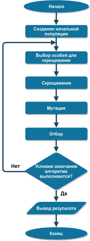
Consider each stage of the algorithm in more detail.

Creating an initial population

The first stage of the algorithm is the creation of an initial population, that is, the creation of a multitude of individuals with different values of chromosome x . As a rule, the initial population is created from individuals with a random chromosome value, while trying to ensure that the chromosome values in the population cover the entire search for a solution relatively evenly, if there are no assumptions about where the global extremum may be.

Instead of a random distribution of chromosomes, you can create chromosomes so that the initial x values are evenly distributed throughout the search area with a given step, which depends on how many individuals will be created at this stage of the algorithm.

The more individuals that are created at this stage, the greater the likelihood that the algorithm will find the right solution, and as the size of the initial population increases, as a rule, fewer iterations of the genetic algorithm (number of generations) are required. However, as the population size grows, an increasing number of calculations of the objective function and the performance of other genetic operations at subsequent stages of the algorithm are required. That is, as the population size increases, the calculation time of one generation increases.

In principle, the size of a population does not have to remain constant throughout the work of the genetic algorithm, often as the generation number increases, the population size can be reduced, since Over time, an increasing number of individuals will be located closer to the desired solution. However, the population size is often kept roughly constant.

Selection of individuals for crossing

After the population has been created, it is necessary to determine which individuals will participate in the cross-breeding operation (see the next paragraph). For this stage there are various algorithms. The easiest of them is to cross each individual with each, but then in the next stage you will have to perform too many operations of crossing and calculating the values of the objective function.

It is better to give a greater chance of crossing for individuals with more successful chromosomes (with a minimum value of the objective function), and for those individuals whose objective function is more (worse) barred from leaving the offspring.

Thus, at this stage, it is necessary to create pairs of individuals (or not necessarily pairs, if more individuals can participate in the crossing), for which the next step will be a crossing operation.

Here you can also use different algorithms. For example, create pairs at random. Or you can sort individuals by increasing the value of the objective function and create pairs from individuals closer to the beginning of the sorted list (for example, from individuals in the first half of the list, in the first third of the list, etc.) This method is bad because it takes time to sorting individuals.

Often used tournament method. When several individuals are randomly selected for the role of each applicant for crossing, among which the individual with the best value of the objective function is sent to the future pair. And even here you can enter an element of chance, giving a small chance for an individual with the worst value of the objective function to “defeat” an individual with the best value of the objective function. This allows you to maintain a more heterogeneous population, protecting it from degeneration, i.e. from the situation when all individuals have approximately equal chromosome values, which is equivalent to dumping the algorithm to a single extremum, possibly not global.

The result of this operation will be a list of partners for crossing.

Crossbreeding

Crossing is a genetic operation, as a result of which new individuals are created with new chromosome values. New chromosomes are based on the chromosome of the parents. Most often, in the process of crossing one set of partners, one subsidiary is created, but theoretically there may be more subsidiaries.

The crossing algorithm can also be implemented in different ways. If individuals have a chromosome type - a number, then the simplest thing to do is to create a new chromosome as the arithmetic mean or the geometric average of the chromosomes of the parents. For many tasks, this is sufficient, but other algorithms based on bit operations are most often used.

Bitwise crossing works in such a way that the daughter chromosome consists of a part of the bits of one parent and a part of the bits of another parent, as shown in the following figure:

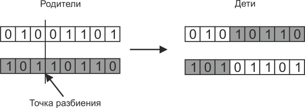
The parent split point is usually chosen randomly. It is not necessary to create two children with such crossing, often limited to one of them.

If the split point of the parent chromosome is one, then such a crossing is called one-point. But you can also use multipoint splitting, when the chromosomes of the parents split into several sections, as shown in the following figure:

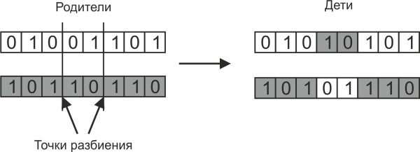
In this case, more combinations of daughter chromosomes are possible.

If the chromosomes are floating point numbers, then all the methods described above can be applied to them, but they will not be very effective. For example, if floating-point numbers are crossed bit-wise, as described earlier, then many crossing operations will create daughter chromosomes that will be different from one of the parents only in the far digit after the decimal point. The situation is especially aggravated if you use double-precision floating-point numbers.

To solve this problem, you need to recall that floating-point numbers according to the IEEE 754 standard are stored as three integers: S (one bit), M, and N, from which the floating-point number is calculated as x = (-1) ^S × M × 2 ^N. One way to cross floating-point numbers is to first split the number into S, M, N, which are integers, and then use the bitwise crossing operations described above to select the S character of one of the parents, and from the obtained values make a daughter chromosome.

In many problems, an individual has not one, but several chromosomes, and it can even be of different types (integers and numbers with a floating point). Then there are even more options for crossing such chromosomes. For example, when creating a daughter individual, all the chromosomes of the parents can be crossed, and some of the chromosomes can be completely transferred from one of the parents unchanged.

Mutation

Mutation is an important stage of the genetic algorithm that maintains the diversity of chromosomes of individuals and thus reduces the chances that the solution will quickly converge to some local minimum instead of a global one. A mutation is a random change in the chromosome of an individual that has just been created by crossing.

As a rule, the probability of a mutation is not established very large, so that the mutation does not interfere with the convergence of the algorithm, otherwise it will spoil the individuals with successful chromosomes.

As well as for crossing, for mutation, you can use different algorithms. For example, it is possible to replace one chromosome or several chromosomes with a random variable. But most often a bit-by-bit mutation is used when one or more bits are inverted into the chromosome (or several chromosomes), as shown in the following figures.

Single bit mutation:

Mutation of several bits:

The number of bits for a mutation can either be set in advance or be a random variable.

As a result, mutations of individuals may turn out to be both more successful and less successful, but this operation allows, with a non-zero probability, a successful chromosome to appear with sets of zeros and ones that the parent did not have.

Selection

As a result of crossing and subsequent mutation, new individuals appear. If there were no selection stage, the number of individuals would grow exponentially, which would require an increasing amount of RAM and time to process each new generation of the population. Therefore, after the appearance of new individuals, it is necessary to clear the population of the least successful individuals. That is what happens at the selection stage.

Selection algorithms can also be different. Often, individuals whose chromosomes do not fall within a specified interval of the search for a solution are rejected first.

Then you can discard the number of the least successful individuals in order to maintain a constant population size. Different probabilistic criteria for selection can also be applied, for example, the probability of selecting an individual can depend on the value of the objective function.

Algorithm End Conditions

As well as in other stages of the genetic algorithm, there are several criteria for the termination of the algorithm.

The simplest criterion for the termination of an algorithm is to interrupt the algorithm after a given iteration number (generation). But this criterion must be used carefully, because the genetic algorithm is probabilistic, and different runs of the algorithm may converge at different speeds. Usually, the termination criterion by iteration number is used as an additional criterion in case the algorithm fails to find a solution for a large number of iterations. Therefore, a sufficiently large number should be set as the threshold of the iteration number.

Another stopping criterion is that the algorithm is interrupted if a new best solution does not appear for a given number of iterations. This means that the algorithm has found a global extremum or is stuck in a local extremum.

There is also an unfavorable situation when the chromosomes of all individuals have the same meaning. This is the so-called degenerate population. Most likely in this case, the algorithm is stuck in one extreme, and not necessarily global. Only a successful mutation can bring a population out of such a state, but since the probability of a mutation is usually determined to be small, and it’s not a fact that the mutation will create a more successful individual, the situation with a degenerate population is usually considered as a reason to stop the genetic algorithm. To check this criterion, it is necessary to compare the chromosomes of all individuals, whether there are differences among them, and if there are no differences, then stop the algorithm.

In some tasks, it is not necessary to find a global minimum, but you need to find a fairly good solution - a solution, the value of the objective function for which is less than a given value. In this case, the algorithm can be stopped ahead of time, if the solution found at the next iteration satisfies this criterion.

optlib

Optlib is a library for the Rust language, designed to optimize functions. At the time of writing these lines, only the genetic algorithm is implemented in the library, but in the future it is planned to expand this library, adding new optimization algorithms to it. Optlib is completely written in Rust.

Optlib is an open source library, distributed under the MIT license.

Page on github - https://github.com/Jenyay/rust-optimization
The page on crates.io is https://crates.io/crates/optlib
Documentation - https://docs.rs/optlib

optlib :: genetic

From the description of the genetic algorithm, it can be seen that many steps of the algorithm can be implemented in different ways, selecting them so that for a given objective function the algorithm converges to the correct solution in the minimum amount of time.

The optlib :: genetic module is designed in such a way that it is possible to assemble a genetic algorithm “from cubes”. When creating an instance of the structure within which the genetic algorithm will work, you need to specify which algorithms will be used to create a population, select partners, cross, mutate, select, and what criteria are used to interrupt the algorithm.

The library already has the most frequently used algorithms for the stages of the genetic algorithm, but you can create your own types that implement the corresponding algorithms.

In the library, the case where the chromosomes are a vector of fractional numbers, that is when the function f ( x ) is minimized, where x is a vector of floating-point numbers ( f32 or f64 ).

Optimization example using optlib :: genetic

Before we begin to describe the genetic module in detail, consider an example of its use to minimize the Schwefel function. This multidimensional function is calculated as follows:

F (b o l d s y m b o l x) = 418.9829 N - s u m_{i = 1}^{N} x_{i} s i n (s q r t | x_{i} |)

$F (\ boldsymbol x) = 418.9829N - \ sum_ {i = 1} ^ {N} x_i \ sin (\ sqrt {| x_i |})$

The minimum of the Schwefel function on the interval -500 <= x _i <= 500 is located at the point x ' , where all x _i = 420.9687 for i = 1, 2, ..., N, and the value of the function at this point f ( x' ) = 0

If N = 2, then the three-dimensional image of this function is as follows:

The extremes are more clearly seen if the lines of the level of this function are plotted:

The following example shows how to find the minimum of the Schwefel function using the genetic module. You can find this example in source codes in the examples / genetic-schwefel folder.

//!    . //! //! y = f(x),  x = (x0, x1, ..., xi,... xn). //!      x' = (420.9687, 420.9687, ...) //!      xi - [-500.0; 500.0]. //! f(x') = 0 //! //! #  //! * ` ` -   . y = f(x). //! * `` -    , x = (x0, x1, x2, ..., xn). //! * `` -   x    . //! * `` -  . //! * `` -    . use optlib::genetic; use optlib::genetic::creation; use optlib::genetic::cross; use optlib::genetic::goal; use optlib::genetic::logging; use optlib::genetic::mutation; use optlib::genetic::pairing; use optlib::genetic::pre_birth; use optlib::genetic::selection; use optlib::genetic::stopchecker; use optlib::testfunctions; use optlib::Optimizer; ///    type Gene = f32; ///   type Chromosomes = Vec<Gene>; fn main() { //   //  .  xi     [-500.0; 500.0] let minval: Gene = -500.0; let maxval: Gene = 500.0; //      let population_size = 500; //   xi  . //  15-   let chromo_count = 15; let intervals = vec![(minval, maxval); chromo_count]; //      ( ) //      optlib::testfunctions let goal = goal::GoalFromFunction::new(testfunctions::schwefel); //       . // RandomCreator       . let creator = creation::vec_float::RandomCreator::new(population_size, intervals.clone()); //        //     . let partners_count = 2; let families_count = population_size / 2; let rounds_count = 5; let pairing = pairing::Tournament::new(partners_count, families_count, rounds_count); //   //      , //   -     let single_cross = cross::FloatCrossExp::new(); let cross = cross::VecCrossAllGenes::new(Box::new(single_cross)); //    //    (     ). let mutation_probability = 15.0; let mutation_gene_count = 3; let single_mutation = mutation::BitwiseMutation::new(mutation_gene_count); let mutation = mutation::VecMutation::new(mutation_probability, Box::new(single_mutation)); // .       , //     . let pre_births: Vec<Box<genetic::PreBirth<Chromosomes>>> = vec![Box::new( pre_birth::vec_float::CheckChromoInterval::new(intervals.clone()), )]; //    //   ,       1e-4 //   3000  (). let stop_checker = stopchecker::CompositeAny::new(vec![ Box::new(stopchecker::Threshold::new(1e-4)), Box::new(stopchecker::MaxIterations::new(3000)), ]); //    .  -   . //        NaN  Inf. //    ,     . let selections: Vec<Box<dyn genetic::Selection<Chromosomes>>> = vec![ Box::new(selection::KillFitnessNaN::new()), Box::new(selection::LimitPopulation::new(population_size)), ]; //     . //       , //       . let loggers: Vec<Box<genetic::Logger<Chromosomes>>> = vec![ Box::new(logging::StdoutResultOnlyLogger::new(15)), Box::new(logging::TimeStdoutLogger::new()), ]; //     let mut optimizer = genetic::GeneticOptimizer::new( Box::new(goal), Box::new(stop_checker), Box::new(creator), Box::new(pairing), Box::new(cross), Box::new(mutation), selections, pre_births, loggers, ); //    optimizer.find_min(); }

This example can be run from the source root by running the command

 cargo run --bin genetic-schwefel --release

The result of the work should look like this:

 Solution: 420.962615966796875 420.940093994140625 420.995391845703125 420.968505859375000 420.950866699218750 421.003784179687500 421.001281738281250 421.300537109375000 421.001708984375000 421.012603759765625 420.880493164062500 420.925079345703125 420.967559814453125 420.999237060546875 421.011505126953125 Goal: 0.015625000000000 Iterations count: 3000 Time elapsed: 2617 ms

A large part of the example code is the creation of type objects for different stages of the genetic algorithm. As it was written at the beginning of the article, each stage of the genetic algorithm can be implemented in various ways. To use the optlib :: lt module, you need to create type objects that implement each stage in one way or another. Then all these objects are transferred to the constructor of the GeneticOptimizer structure, inside which the genetic algorithm is implemented.

The find_min () method of the GeneticOptimizer structure starts the execution of a genetic algorithm.

Basic types and objects

Basic types of the optlib module

The optlib library was developed with a view to the fact that new optimization algorithms will be added in the future, so that the program can easily switch from one optimization algorithm to another, therefore the optlib module contains the Optimizer type, which includes the only method - find_min (), which runs the optimization algorithm for execution. Here the type T is the type of the object that represents a point in the solution search space. For example, in the example above, this is Vec <Gene> (where Gene is an alias for f32). That is, it is the type whose object is input to the objective function.

The Optimizer is declared in the optlib module as follows:

 pub trait Optimizer<T> { fn find_min(&mut self) -> Option<(&T, f64)>; }

The find_min () method of the Optimizer type should return an object of type Option <(& T, f64)>, where & T in the returned tuple is the found solution, and f64 is the value of the objective function for the found solution. If the algorithm could not find a solution, then the find_min () function should return None.

Since many stochastic optimization algorithms use so-called agents (in terms of a genetic algorithm, an agent is an individual), the optlib module also contains the AlgorithmWithAgents type with the only get_agents () method that should return a vector of agents.

The agent, in turn, is a structure that implements one more type from optlib - Agent .

The AlgorithmWithAgents and Agent types are declared in the optlib module as follows:

 pub trait AlgorithmWithAgents<T> { type Agent: Agent<T>; fn get_agents(&self) -> Vec<&Self::Agent>; } pub trait Agent<T> { fn get_parameter(&self) -> &T; fn get_goal(&self) -> f64; }

For both AlgorithmWithAgents and Agent, type T has the same value as Optimizer, that is, it is the type of object for which the value of the objective function is calculated.

GeneticOptimizer structure - implementation of a genetic algorithm

For the structure of GeneticOptimizer both types are implemented - Optimizer and AlgorithmWithAgents.

Each stage of the genetic algorithm is represented by its own type, which can be implemented from scratch or use one of the implementations inside optlib :: genetic. For each stage of the genetic algorithm inside the optlib :: genetic module there is a sub-module with auxiliary structures and functions that implement the most frequently used algorithms of the stages of the genetic algorithm. About these modules will be discussed below. Also inside some of these submodules there is a submodule vec_float that implements the steps of the algorithm for the case if the objective function is calculated from a vector of floating-point numbers (f32 or f64).

The constructor for the GeneticOptimizer structure is declared as follows:

 impl<T: Clone> GeneticOptimizer<T> { pub fn new( goal: Box<dyn Goal<T>>, stop_checker: Box<dyn StopChecker<T>>, creator: Box<dyn Creator<T>>, pairing: Box<dyn Pairing<T>>, cross: Box<dyn Cross<T>>, mutation: Box<dyn Mutation<T>>, selections: Vec<Box<dyn Selection<T>>>, pre_births: Vec<Box<dyn PreBirth<T>>>, loggers: Vec<Box<dyn Logger<T>>>, ) -> GeneticOptimizer<T> { ... } ... }

The constructor GeneticOptimizer accepts a variety of feature objects that affect each stage of the genetic algorithm, as well as the output of the work:

goal: Box <dyn Goal <T >> - objective function;
stop_checker: Box <dyn StopChecker <T >> - stop criterion;
creator: Box <dyn Creator <T >> - creation of the initial population;
pairing: Box <dyn Pairing <T >> - algorithm for choosing partners for crossing;
cross: Box <dyn Cross <T >> - crossing algorithm;
mutation: Box <dyn Mutation <T >> - mutation algorithm;
selections: Vec <Box <dyn Selection <T >>> - vector of selection algorithms;
pre_births: Vec <Box <dyn PreBirth <T >>> - vector of destruction algorithms for unsuccessful chromosomes before creating individuals;
loggers: Vec <Box <dyn Logger <T >>> is a vector of objects that preserve the log of the genetic algorithm.

To run the algorithm, you need to run the find_min () method of the Optimizer type. In addition, the GeneticOptimizer structure has the next_iterations () method, which can be used to continue the calculation after the find_min () method completes.

Sometimes after stopping an algorithm, it is useful to change the parameters of the algorithm or the methods used. This can be done using the following methods of the GeneticOptimizer structure: replace_pairing (), replace_cross (), replace_mutation (), replace_pre_birth (), replace_selection (), replace_stop_checker (). These methods allow you to replace the types of objects that are transferred to the GeneticOptimizer structure when it is created.

The main types for the genetic algorithm are discussed in the following sections.

Description Goal - objective function

The type Goal is declared in the optlib :: genetic module as follows:

 pub trait Goal<T> { fn get(&self, chromosomes: &T) -> f64; }

The get () method must return the value of the objective function for the given chromosome.

Inside the optlib :: genetic :: goal module there is a GoalFromFunction structure that implements the Goal type. For this structure, there is a constructor that accepts a function, which is an objective function. That is, using this structure, you can create a type-object Goal from a normal function.

Description Creator - creating an initial population

Description Creator describes the "creator" of the initial population. This type is declared as follows:

 pub trait Creator<T: Clone> { fn create(&mut self) -> Vec<T>; }

The create () method should return the vector of chromosomes on which the initial population will be created.

For the case if the function of several floating-point numbers is optimized, in the optlib :: genetic :: creator :: vec_float module there is a RandomCreator <G> structure for creating the initial chromosome distribution at random.

Hereinafter, type <G> is the type of one chromosome in the chromosome vector (sometimes the term “gene” is used instead of the term “chromosome”). Generally, the type <G> will be understood as the type f32 or f64 in case the chromosomes are type Vec <f32> or Vec <f64>.

The structure of RandomCreator <G> is declared as follows:

 pub struct RandomCreator<G: Clone + NumCast + PartialOrd> { ... }

Here NumCast is a type from the num crate. This type allows you to create a type from other numeric types using the from () method.

To create the RandomCreator <G> structure, you need to use the new () function, which is declared as follows:

 pub fn new(population_size: usize, intervals: Vec<(G, G)>) -> RandomCreator<G> { ... }

Here population_size is the population size (the number of sets of chromosomes you need to create), and the intervals is the vector of two-element tuples, the minimum and maximum value of the corresponding chromosome (gene) in the set of chromosomes, and the size of this vector determines how many chromosomes each individual.

In the example above, the Schwefel function was optimized for 15 variables of type f32. Each variable must lie in the interval [-500; 500]. That is, to create a population, the interval vector must contain 15 tuples (-500.0f32, 500.0f32).

Type Pairing - the choice of partners for crossing

Type Pairing is used to select individuals that will interbreed with each other. This type is declared as follows:

 pub trait Pairing<T: Clone> { fn get_pairs(&mut self, population: &Population<T>) -> Vec<Vec<usize>>; }

The get_pairs () method borrows a pointer to a Population structure that contains all individuals of a population, and through this structure you can find out the best and worst individuals in a population.

The pairing get_pairs () method of type should return a vector that contains vectors that store indices of individuals that will interbreed with each other. Depending on the crossing algorithm (which will be discussed in the next section), two or more individuals may cross.

For example, if individuals with index 0 and 10, 5 and 2, 6 and 3 are crossed, the get_pairs () method should return the vector vec! [Vec! [0, 10], vec! [5, 2], vec! [ 6, 3]].

The optlib :: genetic :: pairing module contains two structures that implement various partner selection algorithms.

For the RandomPairing structure, the pairing type is implemented in such a way that partners are randomly selected for crossing.

For the Tournament structure, the Pairing type is implemented in such a way that the tournament method is used. The tournament method implies that each individual that will participate in the crossing must defeat another individual (the value of the objective function of the winning individual must be less). If in the tournament method one round is used, this means that two individuals are randomly selected, and an individual with a lower value of the objective function among these two individuals enters the future “family”. If several rounds are used, the winning individual must thus win against several random individuals.

The structure constructor of Tournament is declared as follows:

 pub fn new(partners_count: usize, families_count: usize, rounds_count: usize) -> Tournament { ... }

Here:

partners_count - the required number of individuals for crossing;
families_count is the number of “families”, i.e. sets of individuals that will breed offspring;
rounds_count - the number of rounds in the tournament.

As a further modification of the tournament method, you can use a random number generator to give a small chance to defeat individuals with the worst value of the objective function, i.e. to make sure that the probability of victory was influenced by the value of the objective function, and the greater the difference between the two competitors, the more chances to win the best individual, and with almost equal values of the objective function, the probability of winning one individual would be close to 50%.

Cross Type - Crossing

After the “families” of individuals have been formed, for crossing, you need to cross their chromosomes in order to get children with new chromosomes. The crossing stage is represented by the Cross type, which is announced as follows:

 pub trait Cross<T: Clone> { fn cross(&mut self, parents: &[&T]) -> Vec<T>; }

The cross () method crosses one set of parents. This method takes the parents parameter — a slice from references to the chromosomes of the parents (not the individuals themselves) —and should return a vector from the new chromosomes. Parents size depends on the choice of partners for crossing with the help of the pairing type, which was described in the previous section. Often used an algorithm that creates new chromosomes based on chromosomes from two parents, then the size of parents will be equal to two.

optlib::genetic::cross , Cross .

VecCrossAllGenes — , , — . VecCrossAllGenes - Cross, . . VecCrossAllGenes, — Vec<f32>.
CrossMean — , , , .
FloatCrossGeometricMean is a structure that crosses two numbers in such a way that, as a daughter chromosome, there will be a number calculated as a geometric average from the parent chromosomes. As chromosomes must be floating point numbers.
CrossBitwise - bitwise single-point crossing of two numbers.
FloatCrossExp - bitwise single-point crossing of floating point numbers. Independently mantissa and parent exhibitors intersect. Sign child receives from one of the parents.

The optlib :: genetic :: cross module also contains functions for bit- wisely crossing numbers of different types - integer and floating-point.

Mutation type - mutation

, , . Mutation , :

 pub trait Mutation<T: Clone> { fn mutation(&mut self, chromosomes: &T) -> T; }

mutation() Mutation . , , , , - , .

optlib::genetic::mutation .

, , VecMutation , VecCrossAllGenes , .. — , VecMutation - Mutation , ( -).

optlib::genetic::mutation BitwiseMutation , Mutation. . VecMutation.

PreBirth —

, . optlib::genetic , . , , , . , , [-500; 500].

PreBirth , :

 pub trait PreBirth<T: Clone> { fn pre_birth(&mut self, population: &Population<T>, new_chromosomes: &mut Vec<T>); }

pre_birth() PreBirth Population , new_chromosomes. , . pre_birth() , .

, , optlib::genetic::pre_birth::vec_float CheckChromoInterval , , , - .

CheckChromoInterval :

 pub fn new(intervals: Vec<(G, G)>) -> CheckChromoInterval<G> { ... }

— . , intervals - . intervals 15 (-500.0f32, 500.0f32).

Selection —

( Population ). . , . Selection , :

 pub trait Selection<T: Clone> { fn kill(&mut self, population: &mut Population<T>); }

, Selection, kill() kill() Individual () , .

, IterMut() Population.

, GeneticOptimizer , - Selection.

, optlib::genetic::selection .

KillFitnessNaN — , NaN Inf.
LimitPopulation — , .
optlib::genetic::selection::vec_float::CheckChromoInterval — , , , . optlib::genetic::pre_birth::vec_floatCheckChromoInterval .

StopChecker —

, . , . , StopChecker , :

 pub trait StopChecker<T: Clone> { fn can_stop(&mut self, population: &Population<T>) -> bool; }

can_stop() true, , false.

optlib::genetic::stopchecker :

MaxIterations — . ().
GoalNotChange — , , . , .
Threshold — , , .
CompositeAll — , ( - StopChecker). , - , .
CompositeAny — , ( - StopChecker). , - , .

Logger —

Logger , , , . Logger :

 pub trait Logger<T: Clone> { ///       fn start(&mut self, _population: &Population<T>) {} ///     , ///           fn resume(&mut self, _population: &Population<T>) {} ///         /// (    ) fn next_iteration(&mut self, _population: &Population<T>) {} ///      fn finish(&mut self, _population: &Population<T>) {} }

optlib::genetic::logging , Logger:

StdoutResultOnlyLogger - after the algorithm is completed, it displays the result of the operation in the console;
VerboseStdoutLogger - at the end of each iteration, the best solution for this iteration is the solution and the value of the objective function for it.
TimeStdoutLogger - at the end of the execution of the algorithm, displays the time that the calculation took to the console.

The constructor of the GeneticOptimizer structure takes as its last argument a vector of type Logger objects, which allows you to flexibly customize the output of the program.

Options for testing optimization algorithms

Schwefel function

. optlib::testfunctions , . optlib::testfunctions .

— , . , :

F (x) = 418.9829 N - \sum_{i = 1}^{N} x_{i} \sin (\sqrt{| x_{i} |})

$F(\boldsymbol x) = 418.9829N - \sum_{i=1}^{N}x_i \sin (\sqrt{|x_i|})$

x' = (420.9687, 420.9687, ...). .

optlib::testfunctions schwefel . N .

, , , , .

F (x) = \sum_{i = 1}^{N} (x_{i} - n)^{2}

$F(\boldsymbol x) = \sum_{i=1}^{N} (x_i - n)^2$

x' = (1.0, 2.0,… N). .

optlib::testfunctions paraboloid .

Conclusion

optlib , . ( optlib::genetic ), , , , .

optlib::genetic. . , , , , .

, . , ( , ..)

In addition, it is planned to add new analytical functions (in addition to the Schwefel function) for testing optimization algorithms.

Once again I will remind links related to the optlib library:

Page on github - https://github.com/Jenyay/rust-optimization
The page on crates.io is https://crates.io/crates/optlib
Documentation - https://docs.rs/optlib

Waiting for your comments, additions and comments.

Source: https://habr.com/ru/post/448870/

All Articles