About removing a trend from experimental data
When analyzing experimentally obtained stationary time series, as a rule, during preliminary preparation (preprocessing) of data, it becomes necessary to suppress the trend existing in them.
Here a “new” trend selection method will be proposed - a simple, obvious and suitable for very complex types of trend.
The trend is usually understood as an ultra-low-frequency non-harmonic component that sharply violates the stationarity of the process. The most common cause of the trend in the experimentally obtained data is the “zero drift” of the recording equipment. Integration of data and some other types of processing can also cause a trend. The presence of a trend greatly distorts the results of subsequent data processing (spectral estimation, etc.), therefore, the removal of the trend is necessary. In some cases, the trend itself is a valuable source of information (for example, when analyzing long-term trends in economic or weather processes).
')
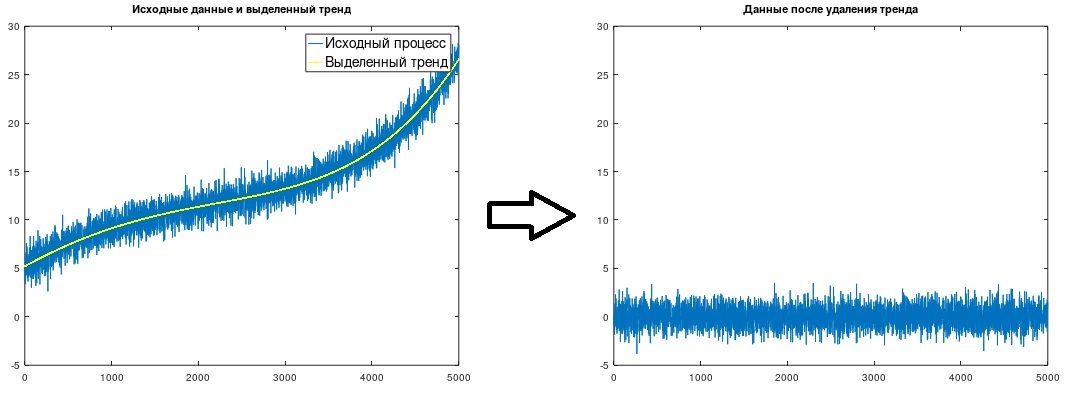
Fig. 1. Isolation and removal of the trend
Usually, a trend is modeled using linear or power (2nd or 3rd order) functions, the coefficients of which are calculated by multiplying the process by certain sequences and then applying rather complex formulas derived from the least squares method. (See, for example, J. Bendat, A. Pirsol, “Applied analysis of random data,” M., Mir, 1989.) The following is a slightly modified method, also based on the least squares method, which is very simple to understand and learn. and does not require reference to the directories, nor independent complex symbolic calculations to obtain the necessary dependencies, while allowing you to simulate the trend with functions of any kind. This modified method is so simple and obvious (once mastered, the scripts can then be written from memory) that they probably have been “invented” more than once by various researchers, but so far I have not come across anything in any sources.
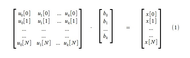
To highlight the trend, an approximation of the initial process x [i] consisting of N + 1 counts is performed using a small number k of the trend components of the functions u j [i]:
(Usually, the functions u j [i] are chosen as functions of powers,

but for this method it is absolutely unprincipled)
The system of linear algebraic equations (1) includes k unknown b j and N + 1 equations.
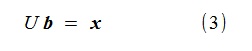
Taking the notation:

write more compactly
The application of the method of least squares when searching for an approximate solution of an overdetermined system, is written in matrix form as follows:

When writing a script: Naturally, there is no need to store the entire large matrix U, the elements of the matrix U T U and the vector U T x can be “accumulated” step by step.
System (4) of k equations and k unknowns is solved by obvious methods — well, for example, we write this:

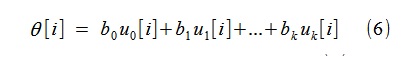
then, by finding b j , you can build a trend θ [i] in the form
For example, a random process x [i] was modeled
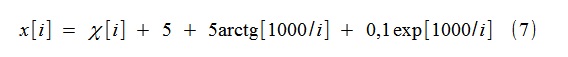
where χ [i] is Gaussian white noise with unit variance. The trend is modeled by functions of type (2) (more precisely, (8)), up to the 4th order inclusive (k = 4).
When using power functions to model a trend, it should be noted that the matrix U T U (4) is theoretically always reversible due to the linear independence of these functions, but at high orders of k (or very long realizations N, which is less critical), certain elements of it can be great in absolute value. For high orders of k, in the case of computational difficulties, it is recommended to use decreasing coefficients, for example, such (8):

(Δt = 1), which was done in the considered example. The trend shown in Fig.1.
After highlighting a trend, naturally, it should simply be subtracted from the original data.
Comment. Usually, authoritative sources do not recommend working with trend models of order higher than k = 2 (square parabola). Whether this is connected with the difficulty of determining the “amplitude” coefficients b j by traditional methods, or with the above-mentioned exhaustion of the orders of machine variables, or with the false assignment to the trend of informative components of the process, is not very clear. In the above example, the trend of the 4th order seems to be quite plausible (though not much different from the trend of the 3rd order). For particularly difficult cases, sources recommend using a different method - low-frequency filtering (not considered here).
Selection of a trend, as shown above — the procedure is not so complicated; it allows you to either isolate and analyze “slow” trends, or, more often, help to get “output” qualitative data - a centered stationary random process suitable for further analysis.
Here a “new” trend selection method will be proposed - a simple, obvious and suitable for very complex types of trend.
The trend is usually understood as an ultra-low-frequency non-harmonic component that sharply violates the stationarity of the process. The most common cause of the trend in the experimentally obtained data is the “zero drift” of the recording equipment. Integration of data and some other types of processing can also cause a trend. The presence of a trend greatly distorts the results of subsequent data processing (spectral estimation, etc.), therefore, the removal of the trend is necessary. In some cases, the trend itself is a valuable source of information (for example, when analyzing long-term trends in economic or weather processes).
')
Fig. 1. Isolation and removal of the trend
Usually, a trend is modeled using linear or power (2nd or 3rd order) functions, the coefficients of which are calculated by multiplying the process by certain sequences and then applying rather complex formulas derived from the least squares method. (See, for example, J. Bendat, A. Pirsol, “Applied analysis of random data,” M., Mir, 1989.) The following is a slightly modified method, also based on the least squares method, which is very simple to understand and learn. and does not require reference to the directories, nor independent complex symbolic calculations to obtain the necessary dependencies, while allowing you to simulate the trend with functions of any kind. This modified method is so simple and obvious (once mastered, the scripts can then be written from memory) that they probably have been “invented” more than once by various researchers, but so far I have not come across anything in any sources.
To highlight the trend, an approximation of the initial process x [i] consisting of N + 1 counts is performed using a small number k of the trend components of the functions u j [i]:
(Usually, the functions u j [i] are chosen as functions of powers,
but for this method it is absolutely unprincipled)
The system of linear algebraic equations (1) includes k unknown b j and N + 1 equations.
Taking the notation:
write more compactly
The application of the method of least squares when searching for an approximate solution of an overdetermined system, is written in matrix form as follows:
When writing a script: Naturally, there is no need to store the entire large matrix U, the elements of the matrix U T U and the vector U T x can be “accumulated” step by step.
System (4) of k equations and k unknowns is solved by obvious methods — well, for example, we write this:
then, by finding b j , you can build a trend θ [i] in the form
For example, a random process x [i] was modeled
where χ [i] is Gaussian white noise with unit variance. The trend is modeled by functions of type (2) (more precisely, (8)), up to the 4th order inclusive (k = 4).
When using power functions to model a trend, it should be noted that the matrix U T U (4) is theoretically always reversible due to the linear independence of these functions, but at high orders of k (or very long realizations N, which is less critical), certain elements of it can be great in absolute value. For high orders of k, in the case of computational difficulties, it is recommended to use decreasing coefficients, for example, such (8):
(Δt = 1), which was done in the considered example. The trend shown in Fig.1.
After highlighting a trend, naturally, it should simply be subtracted from the original data.
Comment. Usually, authoritative sources do not recommend working with trend models of order higher than k = 2 (square parabola). Whether this is connected with the difficulty of determining the “amplitude” coefficients b j by traditional methods, or with the above-mentioned exhaustion of the orders of machine variables, or with the false assignment to the trend of informative components of the process, is not very clear. In the above example, the trend of the 4th order seems to be quite plausible (though not much different from the trend of the 3rd order). For particularly difficult cases, sources recommend using a different method - low-frequency filtering (not considered here).
Selection of a trend, as shown above — the procedure is not so complicated; it allows you to either isolate and analyze “slow” trends, or, more often, help to get “output” qualitative data - a centered stationary random process suitable for further analysis.
Source: https://habr.com/ru/post/448848/
All Articles