Douglas-Pecker Algorithm

Foreword

Not so long ago, we had to work with the simplification of a polygonal chain (a process that allows us to reduce the number of points of a polyline ). In general, this type of task is very common when processing vector graphics and when building maps. As an example, we can take a chain, several points of which fall into the same pixel - it is obvious that all these points can be simplified into one. Some time ago I practically did not know anything about it from the word “absolutely”, in connection with which, I had to quickly fill up the necessary knowledge on this topic. But what was my surprise when I did not find enough comprehensive guides on this issue on the Internet ... I had to search for information from completely different sources with excerpts and, after analysis, build everything into the big picture. Lesson is not the most enjoyable, to be honest. Therefore, I would like to write a series of articles on polygon chain simplification algorithms. I decided to start with the most popular Douglas-Pecker algorithm.

Description

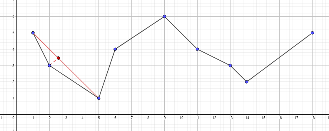
The algorithm specifies the original polyline and the maximum distance (ε) that can be between the original and simplified polylines (that is, the maximum distance from the points of the original to the nearest section of the polyline). The algorithm recursively divides the polyline. The algorithm input is the coordinates of all points between the first and last, including them, as well as the value of ε. The first and last point remain unchanged. After that, the algorithm finds the point furthest from the segment consisting of the first and last ( the search algorithm is the distance from the point to the segment ). If a point is located at a distance less than ε, then all points that have not yet been marked for preservation can be thrown out of the set, and the resulting straight line smoothes the curve with an accuracy not lower than ε. If this distance is greater than ε, then the algorithm recursively calls itself on the set from the starting point to the given and from the given to the ending points. It is worth noting that the Douglas-Pecker algorithm in the course of its work does not preserve the topology. This means that as a result we can get a line with self-intersections. As an illustrative example, take a polyline with the following set of points: [{1; 5}, {2; 3}, {5; sixteen; 4}, {9; 6}, {11; 4}, {13; 3}, {14; 2}, {18; 5}] and look at the process of simplification for different values ​​of ε:

Source polyline from the presented set of points:
')


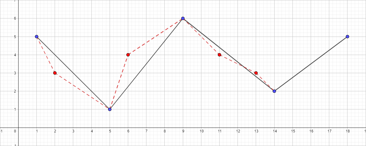
Polyline with ε equal to 0.5:



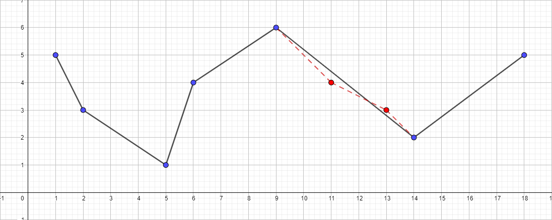
Polyline with ε equal to 1:



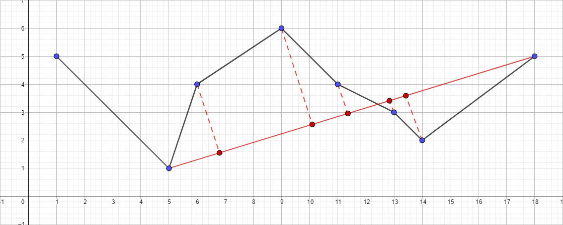
Polyline with ε equal to 1.5:



You can continue to continue to increase the maximum distance and visualization of the algorithm, but I think the main point after these examples has become clear.

Implementation

C ++ was chosen as the programming language for the implementation of the algorithm; you can see the full source code of the algorithm here . And now directly to the implementation itself:

#define X_COORDINATE 0 #define Y_COORDINATE 1 template<typename T> using point_t = std::pair<T, T>; template<typename T> using line_segment_t = std::pair<point_t<T>, point_t<T>>; template<typename T> using points_t = std::vector<point_t<T>>; template<typename CoordinateType> double get_distance_between_point_and_line_segment(const line_segment_t<CoordinateType>& line_segment, const point_t<CoordinateType>& point) noexcept { const CoordinateType x = std::get<X_COORDINATE>(point); const CoordinateType y = std::get<Y_COORDINATE>(point); const CoordinateType x1 = std::get<X_COORDINATE>(line_segment.first); const CoordinateType y1 = std::get<Y_COORDINATE>(line_segment.first); const CoordinateType x2 = std::get<X_COORDINATE>(line_segment.second); const CoordinateType y2 = std::get<Y_COORDINATE>(line_segment.second); const double double_area = abs((y2-y1)*x - (x2-x1)*y + x2*y1 - y2*x1); const double line_segment_length = sqrt(pow((x2-x1), 2) + pow((y2-y1), 2)); if (line_segment_length != 0.0) return double_area / line_segment_length; else return 0.0; } template<typename CoordinateType> void simplify_points(const points_t<CoordinateType>& src_points, points_t<CoordinateType>& dest_points, double tolerance, std::size_t begin, std::size_t end) { if (begin + 1 == end) return; double max_distance = -1.0; std::size_t max_index = 0; for (std::size_t i = begin + 1; i < end; i++) { const point_t<CoordinateType>& cur_point = src_points.at(i); const point_t<CoordinateType>& start_point = src_points.at(begin); const point_t<CoordinateType>& end_point = src_points.at(end); const double distance = get_distance_between_point_and_line_segment({ start_point, end_point }, cur_point); if (distance > max_distance) { max_distance = distance; max_index = i; } } if (max_distance > tolerance) { simplify_points(src_points, dest_points, tolerance, begin, max_index); dest_points.push_back(src_points.at(max_index)); simplify_points(src_points, dest_points, tolerance, max_index, end); } } template< typename CoordinateType, typename = std::enable_if<std::is_integral<CoordinateType>::value || std::is_floating_point<CoordinateType>::value>::type> points_t<CoordinateType> duglas_peucker(const points_t<CoordinateType>& src_points, double tolerance) noexcept { if (tolerance <= 0) return src_points; points_t<CoordinateType> dest_points{}; dest_points.push_back(src_points.front()); simplify_points(src_points, dest_points, tolerance, 0, src_points.size() - 1); dest_points.push_back(src_points.back()); return dest_points; } 

Well, actually the use of the algorithm itself:

 int main() { points_t<int> source_points{ { 1, 5 }, { 2, 3 }, { 5, 1 }, { 6, 4 }, { 9, 6 }, { 11, 4 }, { 13, 3 }, { 14, 2 }, { 18, 5 } }; points_t<int> simplify_points = duglas_peucker(source_points, 1); return EXIT_SUCCESS; } 

An example of the algorithm

As input, we take the set of points [{1; 5}, {2; 3}, {5; sixteen; 4}, {9; 6}, {11; 4}, {13; 3}, {14; 2}, {18; 5}] and ε equal to 1:

• Find the most distant point from the segment {1; 5} - {18; 5}, this point will be the point {5; one }.
  
  
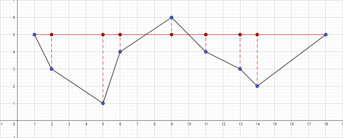
• Check its distance to the segment {1; 5} - {18; five }. It is greater than 1, which means we add it to the resulting polyline.
• Run the recursive algorithm for the segment {1; 5} - {5; 1} and find the furthest point for this segment. This point is {2; 3}.
  
  
• Check its distance to the segment {1; 5} - {5; one }. In this case, it is less than 1, so we can safely drop this point.
• Run the recursive algorithm for the segment {5; 1} - {18; 5} and find the furthest point for this segment ...
  
  
• And so on according to the same plan ...

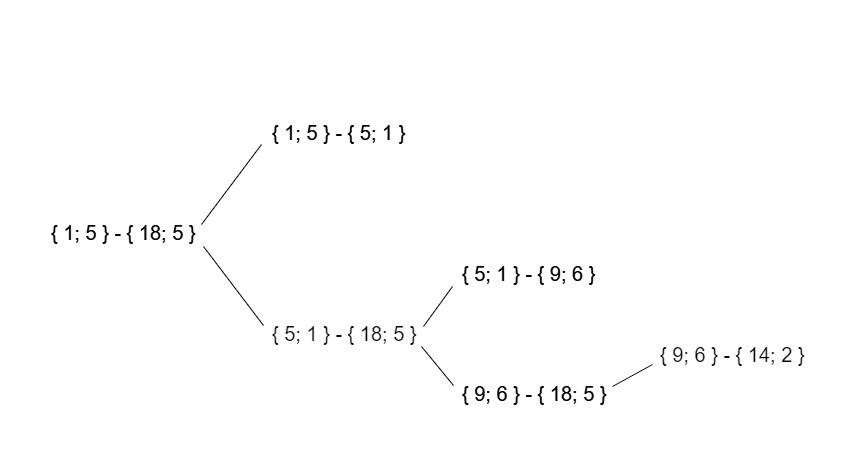
As a result, the recursive call tree for this test data will look like this:

Working hours

The expected complexity of the algorithm is, at best, O (nlogn), this is when the number of the most distant point always turns out to be lexicographically central. However, in the worst case, the complexity of the algorithm is O (n ^ 2). This is achieved, for example, if the number of the most distant point is always adjacent to the number of the boundary point.

I hope that my article will be useful to someone, I would also like to draw attention to the fact that if the article shows sufficient interest among readers, I will soon be ready to consider algorithms for simplifying the polygonal chain of Reumman-Vitcam, Opheim and Lang. Thanks for attention!