Determine the breed of the dog: the full development cycle, from the Python neural network to the application on Google Play
Progress in the field of neural networks in general and pattern recognition in particular, has led to what may seem as if the creation of a neural network application for working with images is a routine task. In a sense, it is - if you came up with an idea related to pattern recognition, do not doubt that someone has already written something like that. All that is required of you is to find the corresponding piece of code in Google and “compile” it with the author.
However, there are still numerous details that make the task not so much unsolvable as ... boring, I would say. It takes too much time, especially if you are a beginner who needs guidance, step by step, a project that is done right before your eyes, and is done from beginning to end. Without the usual in such cases, "skip this obvious part" of excuses.
In this article, we will look at the task of creating a Dog Breed Identifier: create and train a neural network, and then port it to Java for Android and publish it on Google Play.
')
If you want to look at the finished result, here it is: the NeuroDog App on Google Play.
Web site with my robotics (in progress): robotics.snowcron.com .
Web site with the program itself, including the manual: NeuroDog User Guide .
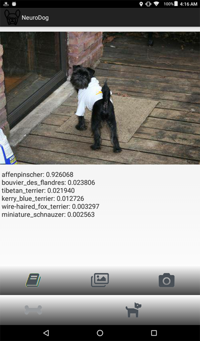
Here is a screenshot of the program:
We will use Keras: a Google library for working with neural networks. This is a high-level library, which means that it is easier to use compared to the alternatives I know. If that - the network has a lot of textbooks on Keras, high quality.
We will use CNN - Convolutional Neural Networks. CNN (and more advanced configurations based on them) are the de facto standard in image recognition. At the same time, it is not always easy to train such a network: it is necessary to choose the right network structure, training parameters (all these learning rate, momentum, L1 and L2, etc.). The task requires significant computational resources, and therefore, to solve it, just sorting through ALL the parameters will not work.
This is one of several reasons why the so-called “transfer knowlege” is used in most cases instead of the so-called “vanilla” approach. Transfer Knowlege uses a neural network trained by someone before us (for example, Google) and usually for a similar, but still different task. We take the initial layers from it, replace the final layers with our own classifier - and it works, moreover, it works perfectly.
At first, a similar result may come as a surprise: how is it that we took a Google network trained to distinguish cats from chairs, and she recognizes us to breed dogs? To understand how this happens, you need to understand the basic principles of the work of Deep Neural Networks, including those used for pattern recognition.
We “fed” the network a picture (an array of numbers, that is) as input. The first layer analyzes the image for simple patterns, such as “horizontal line”, “arc”, etc. The next layer receives these patterns as input, and gives out second-order patterns, like “fur”, “corner of the eye” ... Ultimately, we get a puzzle from which you can reconstruct a dog: wool, two eyes and a human hand in your teeth.
All of the above was done using the pre-trained layers we received (for example, from Google). Next, we add our layers, and teach them to extract information about the breed from these patterns. It sounds logical.
To summarize, in this article we will create both CNN's “vanilla” and several transfer learning options for networks of different types. As for “vanilla”: I’ll create it, but I don’t plan to configure it by selecting parameters, since the “pre-trained” networks are much easier to train and configure.
Since we plan to teach our neural network to recognize dog breeds, we must “show” samples of different breeds to it. Fortunately, there is a set of photos created here for a similar task (the original is here ).
Then I plan to port the best of the received networks under the android. Porting the Kerasov networks for Android is relatively simple, well formalized and we will do all the necessary steps, so it will be easy to reproduce this part.
Then we will post it all on Google Play. Naturally, Google will resist, so that additional tricks will be used. For example, the size of our application (due to the cumbersome neural network) will be larger than the allowed size of the Android APK received by Google Play: we will have to use bundles. In addition, Google will not show our application in the search results, it can be fixed by writing search tags in the application, or just wait ... a week or two.
As a result, we will get a fully functional “commercial” (in quotes, as it is laid out for free) an application for android and using neural networks.
You can program in Keras in different ways, depending on the OS you use (Ubuntu is recommended), the presence or absence of a video card, and so on. There is nothing bad in developing on a local computer (and, accordingly, configuring it), except that this is not the easiest way.
First, installing and configuring a large number of tools and libraries takes time, and then, when new versions come out, you have to spend time again. Secondly, neural networks require large computing power for learning. You can speed up (10 or more times) this process if you are using a GPU ... at the time of this writing, the top GPUs that are most suitable for this job cost 2000 - 7000 dollars. And yes, they also need to be configured.
So we will go the other way. The fact is that Google allows poor hedgehogs like us to use GPUs from their cluster - for free, for calculations related to neural networks, it also provides a fully configured environment, all together, this is called Google Colab. The service gives you access to Jupiter Notebook with python, Keras and a huge number of other libraries already configured. All you need to do is get a Google account (get a Gmail account, and this will give access to everything else).
At the moment, Colab can be found here , but knowing Google, this can change at any time. Just google Google Colab.
An obvious problem with using Colab is that it is a WEB service. How do we get access to our data? Save the neural network after training, for example, download data that is specific to our task, and so on?
There are several (at the time of writing this article - three) different ways, we use the one that I think is the most convenient - we use Google Drive.
Google Drive is a cloud-based datastore that works just like a regular hard drive, and it can be mapped on Google Colab (see the code below). After that, you can work with it as you would with files on a local disk. That is, for example, to get access to photos of dogs for training our neural network, we need to upload them to Google Drive, that's all.
Below I give the code in Python, block by block (from Jupiter Notebook). You can copy this code to your Jupiter Notebook and run it, too, block by block, since blocks can be executed independently (of course, variables defined in the early block may be needed in the latter, but this is an obvious dependency).
First of all, let's mount Google Drive. Only two lines. This code should be executed only once per Colab session (for example, once in 6 hours). If you call it a second time while the session is still “alive”, it will be skipped, since the disk is already mounted.
When you first start, you will be asked to confirm your intentions, there is nothing complicated here. Here's what it looks like:
Completely standard include section; It is possible that some of the included files are not needed, well ... sorry. Also, since I'm going to test different neural networks, you will have to comment / uncomment some of the included modules for specific types of neural networks: for example, to use InceptionV3 NN, uncomment the inclusion of InceptionV3, and comment out, for example, ResNet50. Or not: all that will change is the size of the memory used, and that is not very much.
On Google Drive, we create a folder for our files. The second line displays its contents:
As you can see, photos of dogs (copied from Stanford dataset (see above) on Google Drive) are first stored in the all_images folder. Later, we will copy them into the train, valid and test directories. We will save the trained models in the models folder. As for the labels.csv file, this is part of the dataset with photos, it contains a table of correspondences of the names of pictures and dog breeds.
There are many tests that you can run to understand what we got for temporary use from Google. For example:
As you can see, the GPU is really connected, and if not, you need to find and enable this option in the Jupiter Notebook settings.
Next we need to declare some constants, such as the size of pictures, etc. We will use images of 256x256 pixels, this is a large enough image so as not to lose detail, and small enough to fit everything in memory. Note, however, that some types of neural networks that we will use expect images of 224x224 pixels. In such cases, we comment 256 and uncomment 224.
The same approach (comment one - uncomment) will be applied to the names of the models that we save, simply because we do not want to overwrite files that might still be useful.
First of all, let's load the labels.csv file and split it into the training and validation parts. Notice that there is still no testing part, as I am going to “cheat” to get more data for training.
Next, copy the picture files to the training / validation / testing folders, according to the file names. The following function copies the files that we transfer to the specified folder.
As you can see, we only copy one file to each breed of dogs as test . Also when copying, we create subfolders, one for each breed. Accordingly, the photos are copied to subfolders by breed.
This is done because Keras can work with a directory of a similar structure, loading image files as needed, and not all at once, which saves memory. Uploading all 15,000 pictures at the same time is a bad idea.
We will have to call this function only once, because it copies images - and is no longer needed. Accordingly, for further use, we must comment it out:
We get a list of dog breeds:
We are going to use the Keras library feature called ImageDataGenerators. ImageDataGenerator can process images, scale, rotate, and so on. It can also accept a processing function that can process images additionally.
Note the following code:
We can perform normalization (under the range of data 0-1 instead of the original 0-255) in the ImageDataGenerator itself. Why, then, do we need a preprocessor? As an example, consider (commented out, I do not use it) the call to blur : this is the very custom image manipulation that can be arbitrary. Anything from contrasting to HDR.
We will use two different ImageDataGenerators, one for training and one for validation. The difference is that for training we need turns and scaling to increase the “diversity” of the data, but for validation we don’t need it, at least not in this task.
As already mentioned, we are going to create several types of neural networks. Each time we will call another function to create, include other files and sometimes define a different image size. So, to switch between different types of neural networks, we need comment / uncomment code.
First of all, create CNN's “vanilla”. It works poorly, since I decided not to waste time on fine-tuning it, but at least it provides a basis that can be developed if you want (usually, this is a bad idea, since the pre-trained networks give the best result).
When we create networks using transfer learning , the procedure changes:
Creating networks of other types follows the same pattern:
Attention: winner! This NN showed the best result:
Another one:
Different types of neural networks can be used for different tasks. So, in addition to the requirements of prediction accuracy, size can matter (mobile NN is 5 times smaller than Inception) and speed (if we need to process the video stream in real time, then we have to sacrifice accuracy).
First of all, we are experimenting , so we should be able to remove the neural networks that we have saved, but no longer use. The following function removes the NN if it exists:
The way we create and delete neural networks is quite simple and straightforward. First, delete. When calling delete (only), it should be borne in mind that Jupiter Notebook has a “run selection” function, select only what you want to use, and run.
Then we create a neural network if its file did not exist, or call load if it exists: of course, we cannot call “delete” and then expect NN to exist, so to use the saved neural network, do not call delete .
In other words, we can create a new NN, or use the existing one, depending on the situation and on what we are currently experimenting with. A simple scenario: we trained the neural network, then went on vacation. Returned, and Google nailed the session, so we need to load the previously saved one: comment out “delete” and uncomment “load”.
Checkpoints is a very important element of our program. We can create an array of functions that should be called at the end of each training epoch, and pass it to a checkpoint. For example, you can save a neural network if it shows results that are better than those already saved.
Finally, we learn the neural network on the training set:
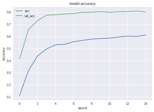
The graphs for accuracy and loss for the best configuration are as follows:

As you can see, the neural network is learning, and quite well.
After the training is completed, we must test the result; for this, NN presented pictures that she had never seen before - the ones that we copied into the testing folder - one for each dog breed.
First of all, we need to organize the loading of the neural network from the disk. The reason is clear: the export takes place in another block of code, so most likely we will start the export separately - when the neural network is brought to the optimal state. That is, right before the export, in the same program run, we will not train the network. If you use the code given here, then there is no difference, the optimal network is picked up to you. But if you learn something of your own, then to train everything again before saving is a waste of time, if you have saved everything before.
For the same reason - in order not to jump on the code - I include the files necessary for export here. No one bothers you to move them to the beginning of the program if your sense of beauty requires it:
A small test after loading the neural network, just to make sure that everything loaded is working:

Next, we need to get the names of the input (input) and output (output) layers of the network (either this way or in the creation function, we must explicitly “name” the layers, which we did not do).
We will use the names of the input and output layers later when we import the neural network into a Java application.
Another code is haunting the network to retrieve this data:
But I do not like it and I do not recommend it.
The following code is exporting Keras Neural Network in pb format, one that we will capture from Android.
The last line prints the structure of the resulting neural network.
The export of neural networks to Android is well formalized and should not cause difficulties. There are, as always, several ways, we use the most (at the time of this writing) popular.
First of all, we use Android Studio to create a new project. We will “cut corners”, because our task is not a textbook on android. So the application will contain only one activity.
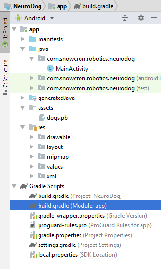
As you can see, we added a folder of “assets” and copied our neural network into it (the one that we previously exported).
There are several changes to this file. First of all, we need to import the tensorflow-android library . It is used to work with Tensorflow (and, accordingly, Keras) from Java:
Another non-obvious stumbling block: versionCode and versionName . When the application changes, you will need to upload new versions on Google Play. Without changing the versions in gdadle (for example, 1 -> 2 -> 3 ...) you cannot do this, Google will give the error "this version is already there."
First of all, our application will be “heavy” - 100 Mb Neural Network will easily fit into the memory of modern cell phones, but opening a separate instance for each photo “shared” from Facebook is definitely a bad idea.
So we prohibit creating more than one instance of our application:
By adding android: launchMode = "singleTask" to MainActivity, we tell Android to open (activate) an existing copy of the application, instead of creating another instance.
Then we need to include our application in the list that the system shows when someone “shares” the picture:
Finally, we need to request the features and permissions our application will use:
If you are familiar with Android programming, this part should not raise questions.
We will create two layouts, one for portrait and one for landscape orientation. It looks like a portrait layout .
What we will do is: a large field (view) to show a picture, an annoying list of ads (shown when the button with a “bone” is pressed), the “Help” button, buttons for downloading a picture from File / Gallery and capturing from the camera, and finally (initially hidden) “Process” button for image processing.
The activity itself contains all the logic of showing and hiding, as well as enabling / disabling buttons, depending on the state of the application.
This activity inherits (extends) the standard Android Activity:
Consider the code responsible for the operation of the neural network.
First of all, the neural network accepts bitmap. Initially, this is a large Bitmap (arbitrary size) from a camera or from a file (m_bitmap), then we transform it, resulting in a standard 256x256 pixels (m_bitmapForNn). We also store the size of bitmap (256) in a constant:
We must tell the neural network the names of the input and output layers; we received them earlier (see listing), but keep in mind that in your case they may differ:
Then we declare a variable to hold the TensofFlow object. Also, we store the path to the neural network file (which lies in the assets):
Breeds of dogs are stored in the list in order to show them to the user, and not array indices:
Initially, we downloaded a bitmap. However, the neural network expects an array of RGB values, and its output is an array of probabilities that this breed is what is shown in the picture. Accordingly, we need to add two more arrays (note that 120 is the number of dog breeds present in our training data):
Load the tensorflow inference library:
Since neural network operations take time, we need to execute them in a separate thread, otherwise there is a chance that we will receive a system message “the application does not respond”, to mention the disgruntled user.
In the onCreate () of the MainActivity, we need to add the onClickListener for the "Process" button:
Here processImage () just calls the thread we described above:
We do not plan to discuss the details of UI programming for Android, since this is absolutely not related to the task of porting neural networks. However, one thing still mention.
When we prevented the creation of additional instances of our application, we also broke down the normal order of creating and deleting activity (flow of control): if you “share” the image from Facebook and then share another one, the application will not restart. This means that the “traditional” way of catching the transferred data in onCreate will not be enough, since onCreate will not be invoked.
Here's how to solve this problem:
1. In the onCreate in MainActivity, we call the onSharedIntent function:
Also add a handler for onNewIntent:
Here is the onSharedIntent function itself:
Now we process the transferred data in onCreate (if the application was not in memory) or in onNewIntent (if it was launched earlier).
Good luck!If you liked the article, please “like” it in all possible ways, there are also “social” buttons on the site .
However, there are still numerous details that make the task not so much unsolvable as ... boring, I would say. It takes too much time, especially if you are a beginner who needs guidance, step by step, a project that is done right before your eyes, and is done from beginning to end. Without the usual in such cases, "skip this obvious part" of excuses.
In this article, we will look at the task of creating a Dog Breed Identifier: create and train a neural network, and then port it to Java for Android and publish it on Google Play.
')
If you want to look at the finished result, here it is: the NeuroDog App on Google Play.
Web site with my robotics (in progress): robotics.snowcron.com .
Web site with the program itself, including the manual: NeuroDog User Guide .
Here is a screenshot of the program:
Formulation of the problem
We will use Keras: a Google library for working with neural networks. This is a high-level library, which means that it is easier to use compared to the alternatives I know. If that - the network has a lot of textbooks on Keras, high quality.
We will use CNN - Convolutional Neural Networks. CNN (and more advanced configurations based on them) are the de facto standard in image recognition. At the same time, it is not always easy to train such a network: it is necessary to choose the right network structure, training parameters (all these learning rate, momentum, L1 and L2, etc.). The task requires significant computational resources, and therefore, to solve it, just sorting through ALL the parameters will not work.
This is one of several reasons why the so-called “transfer knowlege” is used in most cases instead of the so-called “vanilla” approach. Transfer Knowlege uses a neural network trained by someone before us (for example, Google) and usually for a similar, but still different task. We take the initial layers from it, replace the final layers with our own classifier - and it works, moreover, it works perfectly.
At first, a similar result may come as a surprise: how is it that we took a Google network trained to distinguish cats from chairs, and she recognizes us to breed dogs? To understand how this happens, you need to understand the basic principles of the work of Deep Neural Networks, including those used for pattern recognition.
We “fed” the network a picture (an array of numbers, that is) as input. The first layer analyzes the image for simple patterns, such as “horizontal line”, “arc”, etc. The next layer receives these patterns as input, and gives out second-order patterns, like “fur”, “corner of the eye” ... Ultimately, we get a puzzle from which you can reconstruct a dog: wool, two eyes and a human hand in your teeth.
All of the above was done using the pre-trained layers we received (for example, from Google). Next, we add our layers, and teach them to extract information about the breed from these patterns. It sounds logical.
To summarize, in this article we will create both CNN's “vanilla” and several transfer learning options for networks of different types. As for “vanilla”: I’ll create it, but I don’t plan to configure it by selecting parameters, since the “pre-trained” networks are much easier to train and configure.
Since we plan to teach our neural network to recognize dog breeds, we must “show” samples of different breeds to it. Fortunately, there is a set of photos created here for a similar task (the original is here ).
Then I plan to port the best of the received networks under the android. Porting the Kerasov networks for Android is relatively simple, well formalized and we will do all the necessary steps, so it will be easy to reproduce this part.
Then we will post it all on Google Play. Naturally, Google will resist, so that additional tricks will be used. For example, the size of our application (due to the cumbersome neural network) will be larger than the allowed size of the Android APK received by Google Play: we will have to use bundles. In addition, Google will not show our application in the search results, it can be fixed by writing search tags in the application, or just wait ... a week or two.
As a result, we will get a fully functional “commercial” (in quotes, as it is laid out for free) an application for android and using neural networks.
Development environment
You can program in Keras in different ways, depending on the OS you use (Ubuntu is recommended), the presence or absence of a video card, and so on. There is nothing bad in developing on a local computer (and, accordingly, configuring it), except that this is not the easiest way.
First, installing and configuring a large number of tools and libraries takes time, and then, when new versions come out, you have to spend time again. Secondly, neural networks require large computing power for learning. You can speed up (10 or more times) this process if you are using a GPU ... at the time of this writing, the top GPUs that are most suitable for this job cost 2000 - 7000 dollars. And yes, they also need to be configured.
So we will go the other way. The fact is that Google allows poor hedgehogs like us to use GPUs from their cluster - for free, for calculations related to neural networks, it also provides a fully configured environment, all together, this is called Google Colab. The service gives you access to Jupiter Notebook with python, Keras and a huge number of other libraries already configured. All you need to do is get a Google account (get a Gmail account, and this will give access to everything else).
At the moment, Colab can be found here , but knowing Google, this can change at any time. Just google Google Colab.
An obvious problem with using Colab is that it is a WEB service. How do we get access to our data? Save the neural network after training, for example, download data that is specific to our task, and so on?
There are several (at the time of writing this article - three) different ways, we use the one that I think is the most convenient - we use Google Drive.
Google Drive is a cloud-based datastore that works just like a regular hard drive, and it can be mapped on Google Colab (see the code below). After that, you can work with it as you would with files on a local disk. That is, for example, to get access to photos of dogs for training our neural network, we need to upload them to Google Drive, that's all.
Creation and training of a neural network
Below I give the code in Python, block by block (from Jupiter Notebook). You can copy this code to your Jupiter Notebook and run it, too, block by block, since blocks can be executed independently (of course, variables defined in the early block may be needed in the latter, but this is an obvious dependency).
Initialization
First of all, let's mount Google Drive. Only two lines. This code should be executed only once per Colab session (for example, once in 6 hours). If you call it a second time while the session is still “alive”, it will be skipped, since the disk is already mounted.
from google.colab import drive drive.mount('/content/drive/') When you first start, you will be asked to confirm your intentions, there is nothing complicated here. Here's what it looks like:
>>> Go to this URL in a browser: ... >>> Enter your authorization code: >>> ·········· >>> Mounted at /content/drive/ Completely standard include section; It is possible that some of the included files are not needed, well ... sorry. Also, since I'm going to test different neural networks, you will have to comment / uncomment some of the included modules for specific types of neural networks: for example, to use InceptionV3 NN, uncomment the inclusion of InceptionV3, and comment out, for example, ResNet50. Or not: all that will change is the size of the memory used, and that is not very much.
import datetime as dt import pandas as pd import seaborn as sns import matplotlib.pyplot as plt from tqdm import tqdm import cv2 import numpy as np import os import sys import random import warnings from sklearn.model_selection import train_test_split import keras from keras import backend as K from keras import regularizers from keras.models import Sequential from keras.models import Model from keras.layers import Dense, Dropout, Activation from keras.layers import Flatten, Conv2D from keras.layers import MaxPooling2D from keras.layers import BatchNormalization, Input from keras.layers import Dropout, GlobalAveragePooling2D from keras.callbacks import Callback, EarlyStopping from keras.callbacks import ReduceLROnPlateau from keras.callbacks import ModelCheckpoint import shutil from keras.applications.vgg16 import preprocess_input from keras.preprocessing import image from keras.preprocessing.image import ImageDataGenerator from keras.models import load_model from keras.applications.resnet50 import ResNet50 from keras.applications.resnet50 import preprocess_input from keras.applications.resnet50 import decode_predictions from keras.applications import inception_v3 from keras.applications.inception_v3 import InceptionV3 from keras.applications.inception_v3 import preprocess_input as inception_v3_preprocessor from keras.applications.mobilenetv2 import MobileNetV2 from keras.applications.nasnet import NASNetMobile On Google Drive, we create a folder for our files. The second line displays its contents:
working_path = "/content/drive/My Drive/DeepDogBreed/data/" !ls "/content/drive/My Drive/DeepDogBreed/data" >>> all_images labels.csv models test train valid As you can see, photos of dogs (copied from Stanford dataset (see above) on Google Drive) are first stored in the all_images folder. Later, we will copy them into the train, valid and test directories. We will save the trained models in the models folder. As for the labels.csv file, this is part of the dataset with photos, it contains a table of correspondences of the names of pictures and dog breeds.
There are many tests that you can run to understand what we got for temporary use from Google. For example:
# Is GPU Working? import tensorflow as tf tf.test.gpu_device_name() >>> '/device:GPU:0' As you can see, the GPU is really connected, and if not, you need to find and enable this option in the Jupiter Notebook settings.
Next we need to declare some constants, such as the size of pictures, etc. We will use images of 256x256 pixels, this is a large enough image so as not to lose detail, and small enough to fit everything in memory. Note, however, that some types of neural networks that we will use expect images of 224x224 pixels. In such cases, we comment 256 and uncomment 224.
The same approach (comment one - uncomment) will be applied to the names of the models that we save, simply because we do not want to overwrite files that might still be useful.
warnings.filterwarnings("ignore") os.environ['TF_CPP_MIN_LOG_LEVEL'] = '2' np.random.seed(7) start = dt.datetime.now() BATCH_SIZE = 16 EPOCHS = 15 TESTING_SPLIT=0.3 # 70/30 % NUM_CLASSES = 120 IMAGE_SIZE = 256 #strModelFileName = "models/ResNet50.h5" # strModelFileName = "models/InceptionV3.h5" strModelFileName = "models/InceptionV3_Sgd.h5" #IMAGE_SIZE = 224 #strModelFileName = "models/MobileNetV2.h5" #IMAGE_SIZE = 224 #strModelFileName = "models/NASNetMobileSgd.h5" Data loading
First of all, let's load the labels.csv file and split it into the training and validation parts. Notice that there is still no testing part, as I am going to “cheat” to get more data for training.
labels = pd.read_csv(working_path + 'labels.csv') print(labels.head()) train_ids, valid_ids = train_test_split(labels, test_size = TESTING_SPLIT) print(len(train_ids), 'train ids', len(valid_ids), 'validation ids') print('Total', len(labels), 'testing images') >>> id breed >>> 0 000bec180eb18c7604dcecc8fe0dba07 boston_bull >>> 1 001513dfcb2ffafc82cccf4d8bbaba97 dingo >>> 2 001cdf01b096e06d78e9e5112d419397 pekinese >>> 3 00214f311d5d2247d5dfe4fe24b2303d bluetick >>> 4 0021f9ceb3235effd7fcde7f7538ed62 golden_retriever >>> 7155 train ids 3067 validation ids >>> Total 10222 testing images Next, copy the picture files to the training / validation / testing folders, according to the file names. The following function copies the files that we transfer to the specified folder.
def copyFileSet(strDirFrom, strDirTo, arrFileNames): arrBreeds = np.asarray(arrFileNames['breed']) arrFileNames = np.asarray(arrFileNames['id']) if not os.path.exists(strDirTo): os.makedirs(strDirTo) for i in tqdm(range(len(arrFileNames))): strFileNameFrom = strDirFrom + arrFileNames[i] + ".jpg" strFileNameTo = strDirTo + arrBreeds[i] + "/" + arrFileNames[i] + ".jpg" if not os.path.exists(strDirTo + arrBreeds[i] + "/"): os.makedirs(strDirTo + arrBreeds[i] + "/") # As a new breed dir is created, copy 1st file # to "test" under name of that breed if not os.path.exists(working_path + "test/"): os.makedirs(working_path + "test/") strFileNameTo = working_path + "test/" + arrBreeds[i] + ".jpg" shutil.copy(strFileNameFrom, strFileNameTo) shutil.copy(strFileNameFrom, strFileNameTo) As you can see, we only copy one file to each breed of dogs as test . Also when copying, we create subfolders, one for each breed. Accordingly, the photos are copied to subfolders by breed.
This is done because Keras can work with a directory of a similar structure, loading image files as needed, and not all at once, which saves memory. Uploading all 15,000 pictures at the same time is a bad idea.
We will have to call this function only once, because it copies images - and is no longer needed. Accordingly, for further use, we must comment it out:
# Move the data in subfolders so we can # use the Keras ImageDataGenerator. # This way we can also later use Keras # Data augmentation features. # --- Uncomment once, to copy files --- #copyFileSet(working_path + "all_images/", # working_path + "train/", train_ids) #copyFileSet(working_path + "all_images/", # working_path + "valid/", valid_ids) We get a list of dog breeds:
breeds = np.unique(labels['breed']) map_characters = {} #{0:'none'} for i in range(len(breeds)): map_characters[i] = breeds[i] print("<item>" + breeds[i] + "</item>") >>> <item>affenpinscher</item> >>> <item>afghan_hound</item> >>> <item>african_hunting_dog</item> >>> <item>airedale</item> >>> <item>american_staffordshire_terrier</item> >>> <item>appenzeller</item> Image processing
We are going to use the Keras library feature called ImageDataGenerators. ImageDataGenerator can process images, scale, rotate, and so on. It can also accept a processing function that can process images additionally.
def preprocess(img): img = cv2.resize(img, (IMAGE_SIZE, IMAGE_SIZE), interpolation = cv2.INTER_AREA) # or use ImageDataGenerator( rescale=1./255... img_1 = image.img_to_array(img) img_1 = cv2.resize(img_1, (IMAGE_SIZE, IMAGE_SIZE), interpolation = cv2.INTER_AREA) img_1 = np.expand_dims(img_1, axis=0) / 255. #img = cv2.blur(img,(5,5)) return img_1[0] Note the following code:
# or use ImageDataGenerator( rescale=1./255... We can perform normalization (under the range of data 0-1 instead of the original 0-255) in the ImageDataGenerator itself. Why, then, do we need a preprocessor? As an example, consider (commented out, I do not use it) the call to blur : this is the very custom image manipulation that can be arbitrary. Anything from contrasting to HDR.
We will use two different ImageDataGenerators, one for training and one for validation. The difference is that for training we need turns and scaling to increase the “diversity” of the data, but for validation we don’t need it, at least not in this task.
train_datagen = ImageDataGenerator( preprocessing_function=preprocess, #rescale=1./255, # done in preprocess() # randomly rotate images (degrees, 0 to 30) rotation_range=30, # randomly shift images horizontally # (fraction of total width) width_shift_range=0.3, height_shift_range=0.3, # randomly flip images horizontal_flip=True, ,vertical_flip=False, zoom_range=0.3) val_datagen = ImageDataGenerator( preprocessing_function=preprocess) train_gen = train_datagen.flow_from_directory( working_path + "train/", batch_size=BATCH_SIZE, target_size=(IMAGE_SIZE, IMAGE_SIZE), shuffle=True, class_mode="categorical") val_gen = val_datagen.flow_from_directory( working_path + "valid/", batch_size=BATCH_SIZE, target_size=(IMAGE_SIZE, IMAGE_SIZE), shuffle=True, class_mode="categorical") Creating a neural network
As already mentioned, we are going to create several types of neural networks. Each time we will call another function to create, include other files and sometimes define a different image size. So, to switch between different types of neural networks, we need comment / uncomment code.
First of all, create CNN's “vanilla”. It works poorly, since I decided not to waste time on fine-tuning it, but at least it provides a basis that can be developed if you want (usually, this is a bad idea, since the pre-trained networks give the best result).
def createModelVanilla(): model = Sequential() # Note the (7, 7) here. This is one of technics # used to reduce memory use by the NN: we scan # the image in a larger steps. # Also note regularizers.l2: this technic is # used to prevent overfitting. The "0.001" here # is an empirical value and can be optimized. model.add(Conv2D(16, (7, 7), padding='same', use_bias=False, input_shape=(IMAGE_SIZE, IMAGE_SIZE, 3), kernel_regularizer=regularizers.l2(0.001))) # Note the use of a standard CNN building blocks: # Conv2D - BatchNormalization - Activation # MaxPooling2D - Dropout # The last two are used to avoid overfitting, also, # MaxPooling2D reduces memory use. model.add(BatchNormalization(axis=3, scale=False)) model.add(Activation("relu")) model.add(MaxPooling2D(pool_size=(2, 2), strides=(2, 2), padding='same')) model.add(Dropout(0.5)) model.add(Conv2D(16, (3, 3), padding='same', use_bias=False, kernel_regularizer=regularizers.l2(0.01))) model.add(BatchNormalization(axis=3, scale=False)) model.add(Activation("relu")) model.add(MaxPooling2D(pool_size=(2, 2), strides=(1, 1), padding='same')) model.add(Dropout(0.5)) model.add(Conv2D(32, (3, 3), padding='same', use_bias=False, kernel_regularizer=regularizers.l2(0.01))) model.add(BatchNormalization(axis=3, scale=False)) model.add(Activation("relu")) model.add(Dropout(0.5)) model.add(Conv2D(32, (3, 3), padding='same', use_bias=False, kernel_regularizer=regularizers.l2(0.01))) model.add(BatchNormalization(axis=3, scale=False)) model.add(Activation("relu")) model.add(MaxPooling2D(pool_size=(2, 2), strides=(1, 1), padding='same')) model.add(Dropout(0.5)) model.add(Conv2D(64, (3, 3), padding='same', use_bias=False, kernel_regularizer=regularizers.l2(0.01))) model.add(BatchNormalization(axis=3, scale=False)) model.add(Activation("relu")) model.add(Dropout(0.5)) model.add(Conv2D(64, (3, 3), padding='same', use_bias=False, kernel_regularizer=regularizers.l2(0.01))) model.add(BatchNormalization(axis=3, scale=False)) model.add(Activation("relu")) model.add(MaxPooling2D(pool_size=(2, 2), strides=(1, 1), padding='same')) model.add(Dropout(0.5)) model.add(Conv2D(128, (3, 3), padding='same', use_bias=False, kernel_regularizer=regularizers.l2(0.01))) model.add(BatchNormalization(axis=3, scale=False)) model.add(Activation("relu")) model.add(Dropout(0.5)) model.add(Conv2D(128, (3, 3), padding='same', use_bias=False, kernel_regularizer=regularizers.l2(0.01))) model.add(BatchNormalization(axis=3, scale=False)) model.add(Activation("relu")) model.add(MaxPooling2D(pool_size=(2, 2), strides=(1, 1), padding='same')) model.add(Dropout(0.5)) model.add(Conv2D(256, (3, 3), padding='same', use_bias=False, kernel_regularizer=regularizers.l2(0.01))) model.add(BatchNormalization(axis=3, scale=False)) model.add(Activation("relu")) model.add(Dropout(0.5)) model.add(Conv2D(256, (3, 3), padding='same', use_bias=False, kernel_regularizer=regularizers.l2(0.01))) model.add(BatchNormalization(axis=3, scale=False)) model.add(Activation("relu")) model.add(MaxPooling2D(pool_size=(2, 2), strides=(1, 1), padding='same')) model.add(Dropout(0.5)) # This is the end on "convolutional" part of CNN. # Now we need to transform multidementional # data into one-dim. array for a fully-connected # classifier: model.add(Flatten()) # And two layers of classifier itself (plus an # Activation layer in between): model.add(Dense(NUM_CLASSES, activation='softmax', kernel_regularizer=regularizers.l2(0.01))) model.add(Activation("relu")) model.add(Dense(NUM_CLASSES, activation='softmax', kernel_regularizer=regularizers.l2(0.01))) # We need to compile the resulting network. # Note that there are few parameters we can # try here: the best performing one is uncommented, # the rest is commented out for your reference. #model.compile(optimizer='rmsprop', # loss='categorical_crossentropy', # metrics=['accuracy']) #model.compile( # optimizer=keras.optimizers.RMSprop(lr=0.0005), # loss='categorical_crossentropy', # metrics=['accuracy']) model.compile(optimizer='adam', loss='categorical_crossentropy', metrics=['accuracy']) #model.compile(optimizer='adadelta', # loss='categorical_crossentropy', # metrics=['accuracy']) #opt = keras.optimizers.Adadelta(lr=1.0, # rho=0.95, epsilon=0.01, decay=0.01) #model.compile(optimizer=opt, # loss='categorical_crossentropy', # metrics=['accuracy']) #opt = keras.optimizers.RMSprop(lr=0.0005, # rho=0.9, epsilon=None, decay=0.0001) #model.compile(optimizer=opt, # loss='categorical_crossentropy', # metrics=['accuracy']) # model.summary() return(model) When we create networks using transfer learning , the procedure changes:
def createModelMobileNetV2(): # First, create the NN and load pre-trained # weights for it ('imagenet') # Note that we are not loading last layers of # the network (include_top=False), as we are # going to add layers of our own: base_model = MobileNetV2(weights='imagenet', include_top=False, pooling='avg', input_shape=(IMAGE_SIZE, IMAGE_SIZE, 3)) # Then attach our layers at the end. These are # to build "classifier" that makes sense of # the patterns previous layers provide: x = base_model.output x = Dense(512)(x) x = Activation('relu')(x) x = Dropout(0.5)(x) predictions = Dense(NUM_CLASSES, activation='softmax')(x) # Create a model model = Model(inputs=base_model.input, outputs=predictions) # We need to make sure that pre-trained # layers are not changed when we train # our classifier: # Either this: #model.layers[0].trainable = False # or that: for layer in base_model.layers: layer.trainable = False # As always, there are different possible # settings, I tried few and chose the best: # model.compile(optimizer='adam', # loss='categorical_crossentropy', # metrics=['accuracy']) model.compile(optimizer='sgd', loss='categorical_crossentropy', metrics=['accuracy']) #model.summary() return(model) Creating networks of other types follows the same pattern:
def createModelResNet50(): base_model = ResNet50(weights='imagenet', include_top=False, pooling='avg', input_shape=(IMAGE_SIZE, IMAGE_SIZE, 3)) x = base_model.output x = Dense(512)(x) x = Activation('relu')(x) x = Dropout(0.5)(x) predictions = Dense(NUM_CLASSES, activation='softmax')(x) model = Model(inputs=base_model.input, outputs=predictions) #model.layers[0].trainable = False # model.compile(loss='categorical_crossentropy', # optimizer='adam', metrics=['accuracy']) model.compile(optimizer='sgd', loss='categorical_crossentropy', metrics=['accuracy']) #model.summary() return(model) Attention: winner! This NN showed the best result:
def createModelInceptionV3(): # model.layers[0].trainable = False # model.compile(optimizer='sgd', # loss='categorical_crossentropy', # metrics=['accuracy']) base_model = InceptionV3(weights = 'imagenet', include_top = False, input_shape=(IMAGE_SIZE, IMAGE_SIZE, 3)) x = base_model.output x = GlobalAveragePooling2D()(x) x = Dense(512, activation='relu')(x) predictions = Dense(NUM_CLASSES, activation='softmax')(x) model = Model(inputs = base_model.input, outputs = predictions) for layer in base_model.layers: layer.trainable = False # model.compile(optimizer='adam', # loss='categorical_crossentropy', # metrics=['accuracy']) model.compile(optimizer='sgd', loss='categorical_crossentropy', metrics=['accuracy']) #model.summary() return(model) Another one:
def createModelNASNetMobile(): # model.layers[0].trainable = False # model.compile(optimizer='sgd', # loss='categorical_crossentropy', # metrics=['accuracy']) base_model = NASNetMobile(weights = 'imagenet', include_top = False, input_shape=(IMAGE_SIZE, IMAGE_SIZE, 3)) x = base_model.output x = GlobalAveragePooling2D()(x) x = Dense(512, activation='relu')(x) predictions = Dense(NUM_CLASSES, activation='softmax')(x) model = Model(inputs = base_model.input, outputs = predictions) for layer in base_model.layers: layer.trainable = False # model.compile(optimizer='adam', # loss='categorical_crossentropy', # metrics=['accuracy']) model.compile(optimizer='sgd', loss='categorical_crossentropy', metrics=['accuracy']) #model.summary() return(model) Different types of neural networks can be used for different tasks. So, in addition to the requirements of prediction accuracy, size can matter (mobile NN is 5 times smaller than Inception) and speed (if we need to process the video stream in real time, then we have to sacrifice accuracy).
Neural network training
First of all, we are experimenting , so we should be able to remove the neural networks that we have saved, but no longer use. The following function removes the NN if it exists:
# Make sure that previous "best network" is deleted. def deleteSavedNet(best_weights_filepath): if(os.path.isfile(best_weights_filepath)): os.remove(best_weights_filepath) print("deleteSavedNet():File removed") else: print("deleteSavedNet():No file to remove") The way we create and delete neural networks is quite simple and straightforward. First, delete. When calling delete (only), it should be borne in mind that Jupiter Notebook has a “run selection” function, select only what you want to use, and run.
Then we create a neural network if its file did not exist, or call load if it exists: of course, we cannot call “delete” and then expect NN to exist, so to use the saved neural network, do not call delete .
In other words, we can create a new NN, or use the existing one, depending on the situation and on what we are currently experimenting with. A simple scenario: we trained the neural network, then went on vacation. Returned, and Google nailed the session, so we need to load the previously saved one: comment out “delete” and uncomment “load”.
deleteSavedNet(working_path + strModelFileName) #if not os.path.exists(working_path + "models"): # os.makedirs(working_path + "models") # #if not os.path.exists(working_path + # strModelFileName): # model = createModelResNet50() model = createModelInceptionV3() # model = createModelMobileNetV2() # model = createModelNASNetMobile() #else: # model = load_model(working_path + strModelFileName) Checkpoints is a very important element of our program. We can create an array of functions that should be called at the end of each training epoch, and pass it to a checkpoint. For example, you can save a neural network if it shows results that are better than those already saved.
checkpoint = ModelCheckpoint(working_path + strModelFileName, monitor='val_acc', verbose=1, save_best_only=True, mode='auto', save_weights_only=False) callbacks_list = [ checkpoint ] Finally, we learn the neural network on the training set:
# Calculate sizes of training and validation sets STEP_SIZE_TRAIN=train_gen.n//train_gen.batch_size STEP_SIZE_VALID=val_gen.n//val_gen.batch_size # Set to False if we are experimenting with # some other part of code, use history that # was calculated before (and is still in # memory bDoTraining = True if bDoTraining == True: # model.fit_generator does the actual training # Note the use of generators and callbacks # that were defined earlier history = model.fit_generator(generator=train_gen, steps_per_epoch=STEP_SIZE_TRAIN, validation_data=val_gen, validation_steps=STEP_SIZE_VALID, epochs=EPOCHS, callbacks=callbacks_list) # --- After fitting, load the best model # This is important as otherwise we'll # have the LAST model loaded, not necessarily # the best one. model.load_weights(working_path + strModelFileName) # --- Presentation part # summarize history for accuracy plt.plot(history.history['acc']) plt.plot(history.history['val_acc']) plt.title('model accuracy') plt.ylabel('accuracy') plt.xlabel('epoch') plt.legend(['acc', 'val_acc'], loc='upper left') plt.show() # summarize history for loss plt.plot(history.history['loss']) plt.plot(history.history['val_loss']) plt.title('model loss') plt.ylabel('loss') plt.xlabel('epoch') plt.legend(['loss', 'val_loss'], loc='upper left') plt.show() # As grid optimization of NN would take too long, # I did just few tests with different parameters. # Below I keep results, commented out, in the same # code. As you can see, Inception shows the best # results: # Inception: # adam: val_acc 0.79393 # sgd: val_acc 0.80892 # Mobile: # adam: val_acc 0.65290 # sgd: Epoch 00015: val_acc improved from 0.67584 to 0.68469 # sgd-30 epochs: 0.68 # NASNetMobile, adam: val_acc did not improve from 0.78335 # NASNetMobile, sgd: 0.8 The graphs for accuracy and loss for the best configuration are as follows:
As you can see, the neural network is learning, and quite well.
Neural Network Testing
After the training is completed, we must test the result; for this, NN presented pictures that she had never seen before - the ones that we copied into the testing folder - one for each dog breed.
# --- Test j = 0 # Final cycle performs testing on the entire # testing set. for file_name in os.listdir( working_path + "test/"): img = image.load_img(working_path + "test/" + file_name); img_1 = image.img_to_array(img) img_1 = cv2.resize(img_1, (IMAGE_SIZE, IMAGE_SIZE), interpolation = cv2.INTER_AREA) img_1 = np.expand_dims(img_1, axis=0) / 255. y_pred = model.predict_on_batch(img_1) # get 5 best predictions y_pred_ids = y_pred[0].argsort()[-5:][::-1] print(file_name) for i in range(len(y_pred_ids)): print("\n\t" + map_characters[y_pred_ids[i]] + " (" + str(y_pred[0][y_pred_ids[i]]) + ")") print("--------------------\n") j = j + 1 Export neural network to java application
First of all, we need to organize the loading of the neural network from the disk. The reason is clear: the export takes place in another block of code, so most likely we will start the export separately - when the neural network is brought to the optimal state. That is, right before the export, in the same program run, we will not train the network. If you use the code given here, then there is no difference, the optimal network is picked up to you. But if you learn something of your own, then to train everything again before saving is a waste of time, if you have saved everything before.
# Test: load and run model = load_model(working_path + strModelFileName) For the same reason - in order not to jump on the code - I include the files necessary for export here. No one bothers you to move them to the beginning of the program if your sense of beauty requires it:
from keras.models import Model from keras.models import load_model from keras.layers import * import os import sys import tensorflow as tf A small test after loading the neural network, just to make sure that everything loaded is working:
img = image.load_img(working_path + "test/affenpinscher.jpg") #basset.jpg") img_1 = image.img_to_array(img) img_1 = cv2.resize(img_1, (IMAGE_SIZE, IMAGE_SIZE), interpolation = cv2.INTER_AREA) img_1 = np.expand_dims(img_1, axis=0) / 255. y_pred = model.predict(img_1) Y_pred_classes = np.argmax(y_pred,axis = 1) # print(y_pred) fig, ax = plt.subplots() ax.imshow(img) ax.axis('off') ax.set_title(map_characters[Y_pred_classes[0]]) plt.show() Next, we need to get the names of the input (input) and output (output) layers of the network (either this way or in the creation function, we must explicitly “name” the layers, which we did not do).
model.summary() >>> Layer (type) >>> ====================== >>> input_7 (InputLayer) >>> ______________________ >>> conv2d_283 (Conv2D) >>> ______________________ >>> ... >>> dense_14 (Dense) >>> ====================== >>> Total params: 22,913,432 >>> Trainable params: 1,110,648 >>> Non-trainable params: 21,802,784 We will use the names of the input and output layers later when we import the neural network into a Java application.
Another code is haunting the network to retrieve this data:
def print_graph_nodes(filename): g = tf.GraphDef() g.ParseFromString(open(filename, 'rb').read()) print() print(filename) print("=======================INPUT===================") print([n for n in g.node if n.name.find('input') != -1]) print("=======================OUTPUT==================") print([n for n in g.node if n.name.find('output') != -1]) print("===================KERAS_LEARNING==============") print([n for n in g.node if n.name.find('keras_learning_phase') != -1]) print("===============================================") print() #def get_script_path(): # return os.path.dirname(os.path.realpath(sys.argv[0])) But I do not like it and I do not recommend it.
The following code is exporting Keras Neural Network in pb format, one that we will capture from Android.
def keras_to_tensorflow(keras_model, output_dir, model_name,out_prefix="output_", log_tensorboard=True): if os.path.exists(output_dir) == False: os.mkdir(output_dir) out_nodes = [] for i in range(len(keras_model.outputs)): out_nodes.append(out_prefix + str(i + 1)) tf.identity(keras_model.output[i], out_prefix + str(i + 1)) sess = K.get_session() from tensorflow.python.framework import graph_util from tensorflow.python.framework graph_io init_graph = sess.graph.as_graph_def() main_graph = graph_util.convert_variables_to_constants( sess, init_graph, out_nodes) graph_io.write_graph(main_graph, output_dir, name=model_name, as_text=False) if log_tensorboard: from tensorflow.python.tools import import_pb_to_tensorboard import_pb_to_tensorboard.import_to_tensorboard( os.path.join(output_dir, model_name), output_dir) Call these functions to export the neural network:
model = load_model(working_path + strModelFileName) keras_to_tensorflow(model, output_dir=working_path + strModelFileName, model_name=working_path + "models/dogs.pb") print_graph_nodes(working_path + "models/dogs.pb") The last line prints the structure of the resulting neural network.
Creating an Android application using a neural network
The export of neural networks to Android is well formalized and should not cause difficulties. There are, as always, several ways, we use the most (at the time of this writing) popular.
First of all, we use Android Studio to create a new project. We will “cut corners”, because our task is not a textbook on android. So the application will contain only one activity.
As you can see, we added a folder of “assets” and copied our neural network into it (the one that we previously exported).
Gradle file
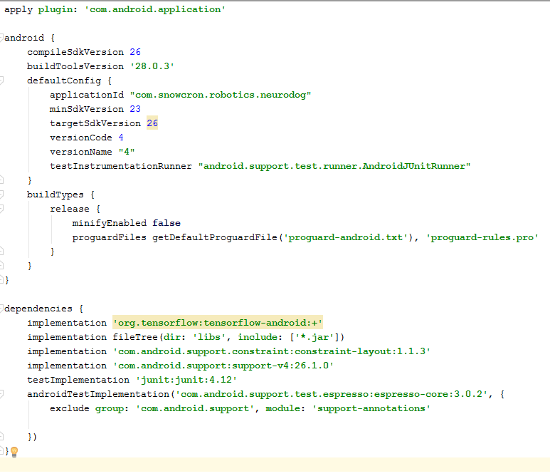
There are several changes to this file. First of all, we need to import the tensorflow-android library . It is used to work with Tensorflow (and, accordingly, Keras) from Java:
Another non-obvious stumbling block: versionCode and versionName . When the application changes, you will need to upload new versions on Google Play. Without changing the versions in gdadle (for example, 1 -> 2 -> 3 ...) you cannot do this, Google will give the error "this version is already there."
Manifesto
First of all, our application will be “heavy” - 100 Mb Neural Network will easily fit into the memory of modern cell phones, but opening a separate instance for each photo “shared” from Facebook is definitely a bad idea.
So we prohibit creating more than one instance of our application:
<activity android:name=".MainActivity" android:launchMode="singleTask"> By adding android: launchMode = "singleTask" to MainActivity, we tell Android to open (activate) an existing copy of the application, instead of creating another instance.
Then we need to include our application in the list that the system shows when someone “shares” the picture:
<intent-filter> <!-- Send action required to display activity in share list --> <action android:name="android.intent.action.SEND" /> <!-- Make activity default to launch --> <category android:name="android.intent.category.DEFAULT" /> <!-- Mime type ie what can be shared with this activity only image and text --> <data android:mimeType="image/*" /> </intent-filter> Finally, we need to request the features and permissions our application will use:
<uses-feature android:name="android.hardware.camera" android:required="true" /> <uses-permission android:name= "android.permission.WRITE_EXTERNAL_STORAGE" /> <uses-permission android:name="android.permission.READ_PHONE_STATE" tools:node="remove" /> If you are familiar with Android programming, this part should not raise questions.
Layout application.
We will create two layouts, one for portrait and one for landscape orientation. It looks like a portrait layout .
What we will do is: a large field (view) to show a picture, an annoying list of ads (shown when the button with a “bone” is pressed), the “Help” button, buttons for downloading a picture from File / Gallery and capturing from the camera, and finally (initially hidden) “Process” button for image processing.
The activity itself contains all the logic of showing and hiding, as well as enabling / disabling buttons, depending on the state of the application.
MainActivity
This activity inherits (extends) the standard Android Activity:
public class MainActivity extends Activity Consider the code responsible for the operation of the neural network.
First of all, the neural network accepts bitmap. Initially, this is a large Bitmap (arbitrary size) from a camera or from a file (m_bitmap), then we transform it, resulting in a standard 256x256 pixels (m_bitmapForNn). We also store the size of bitmap (256) in a constant:
static Bitmap m_bitmap = null; static Bitmap m_bitmapForNn = null; private int m_nImageSize = 256; We must tell the neural network the names of the input and output layers; we received them earlier (see listing), but keep in mind that in your case they may differ:
private String INPUT_NAME = "input_7_1"; private String OUTPUT_NAME = "output_1"; Then we declare a variable to hold the TensofFlow object. Also, we store the path to the neural network file (which lies in the assets):
private TensorFlowInferenceInterface tf;
private String MODEL_PATH =
	"file: ///android_asset/dogs.pb";
Breeds of dogs are stored in the list in order to show them to the user, and not array indices:
private String[] m_arrBreedsArray; Initially, we downloaded a bitmap. However, the neural network expects an array of RGB values, and its output is an array of probabilities that this breed is what is shown in the picture. Accordingly, we need to add two more arrays (note that 120 is the number of dog breeds present in our training data):
private float[] m_arrPrediction = new float[120]; private float[] m_arrInput = null; Load the tensorflow inference library:
static { System.loadLibrary("tensorflow_inference"); } Since neural network operations take time, we need to execute them in a separate thread, otherwise there is a chance that we will receive a system message “the application does not respond”, to mention the disgruntled user.
class PredictionTask extends AsyncTask<Void, Void, Void> { @Override protected void onPreExecute() { super.onPreExecute(); } // --- @Override protected Void doInBackground(Void... params) { try { # We get RGB values packed in integers # from the Bitmap, then break those # integers into individual triplets m_arrInput = new float[ m_nImageSize * m_nImageSize * 3]; int[] intValues = new int[ m_nImageSize * m_nImageSize]; m_bitmapForNn.getPixels(intValues, 0, m_nImageSize, 0, 0, m_nImageSize, m_nImageSize); for (int i = 0; i < intValues.length; i++) { int val = intValues[i]; m_arrInput[i * 3 + 0] = ((val >> 16) & 0xFF) / 255f; m_arrInput[i * 3 + 1] = ((val >> 8) & 0xFF) / 255f; m_arrInput[i * 3 + 2] = (val & 0xFF) / 255f; } // --- tf = new TensorFlowInferenceInterface( getAssets(), MODEL_PATH); //Pass input into the tensorflow tf.feed(INPUT_NAME, m_arrInput, 1, m_nImageSize, m_nImageSize, 3); //compute predictions tf.run(new String[]{OUTPUT_NAME}, false); //copy output into PREDICTIONS array tf.fetch(OUTPUT_NAME, m_arrPrediction); } catch (Exception e) { e.getMessage(); } return null; } // --- @Override protected void onPostExecute(Void result) { super.onPostExecute(result); // --- enableControls(true); // --- tf = null; m_arrInput = null; # strResult contains 5 lines of text # with most probable dog breeds and # their probabilities m_strResult = ""; # What we do below is sorting the array # by probabilities (using map) # and getting in reverse order) the # first five entries TreeMap<Float, Integer> map = new TreeMap<Float, Integer>( Collections.reverseOrder()); for(int i = 0; i < m_arrPrediction.length; i++) map.put(m_arrPrediction[i], i); int i = 0; for (TreeMap.Entry<Float, Integer> pair : map.entrySet()) { float key = pair.getKey(); int idx = pair.getValue(); String strBreed = m_arrBreedsArray[idx]; m_strResult += strBreed + ": " + String.format("%.6f", key) + "\n"; i++; if (i > 5) break; } m_txtViewBreed.setVisibility(View.VISIBLE); m_txtViewBreed.setText(m_strResult); } } In the onCreate () of the MainActivity, we need to add the onClickListener for the "Process" button:
m_btn_process.setOnClickListener(new View.OnClickListener() { @Override public void onClick(View v) { processImage(); } }); Here processImage () just calls the thread we described above:
private void processImage() { try { enableControls(false); // --- PredictionTask prediction_task = new PredictionTask(); prediction_task.execute(); } catch (Exception e) { e.printStackTrace(); } } Additional Notes
We do not plan to discuss the details of UI programming for Android, since this is absolutely not related to the task of porting neural networks. However, one thing still mention.
When we prevented the creation of additional instances of our application, we also broke down the normal order of creating and deleting activity (flow of control): if you “share” the image from Facebook and then share another one, the application will not restart. This means that the “traditional” way of catching the transferred data in onCreate will not be enough, since onCreate will not be invoked.
Here's how to solve this problem:
1. In the onCreate in MainActivity, we call the onSharedIntent function:
protected void onCreate( Bundle savedInstanceState) { super.onCreate(savedInstanceState); .... onSharedIntent(); .... Also add a handler for onNewIntent:
@Override protected void onNewIntent(Intent intent) { super.onNewIntent(intent); setIntent(intent); onSharedIntent(); } Here is the onSharedIntent function itself:
private void onSharedIntent() { Intent receivedIntent = getIntent(); String receivedAction = receivedIntent.getAction(); String receivedType = receivedIntent.getType(); if (receivedAction.equals(Intent.ACTION_SEND)) { // If mime type is equal to image if (receivedType.startsWith("image/")) { m_txtViewBreed.setText(""); m_strResult = ""; Uri receivedUri = receivedIntent.getParcelableExtra( Intent.EXTRA_STREAM); if (receivedUri != null) { try { Bitmap bitmap = MediaStore.Images.Media.getBitmap( this.getContentResolver(), receivedUri); if(bitmap != null) { m_bitmap = bitmap; m_picView.setImageBitmap(m_bitmap); storeBitmap(); enableControls(true); } } catch (Exception e) { e.printStackTrace(); } } } } } Now we process the transferred data in onCreate (if the application was not in memory) or in onNewIntent (if it was launched earlier).
Good luck!If you liked the article, please “like” it in all possible ways, there are also “social” buttons on the site .
Source: https://habr.com/ru/post/448316/
All Articles