About the proximity of the peaks
“Before you comprehend it, it seems like a miracle. But after it there is nothing special. "
No, not about the mountains - about the graphs. There are questions in mathematics, the wording of which is accessible to everyone, but the solution is nontrivial and difficult to explain without special training. One of the problems of this kind can be briefly expressed in the following way - how can we correctly calculate the distances in directed graphs? This somewhat abstract problem can be reduced to a very specific motivating problem. It fits in one picture:
A small town is divided (for example, by a river, although in the context of the peaks a gorge is more suitable) into two districts (parts) A and B . The communication between the districts is carried out along a single road (bridge), which has two lanes: aside from A to B and back. In connection with the growth of the population, the question arose of increasing the capacity of the road. Money as usual is tight and only enough for one lane in one direction. It is clear that even one lane will bring the regions closer together, but the question is how exactly? You are acrazy urban mathematician, and it was you who were invited to get an informed answer.
Instead ofKoenigsberg bridges, one can use a slightly more rigorous language of graph theory. So, there is a directed graph with two vertices (nodes) A and B . The magnitude of the connection (conductivity, throughput) in the forward and reverse directions are initially equal. The question is - how much the distance between the nodes will change if the conduction in one direction is doubled?
')
And yes, if you are a realwelder mathematician, then you can offer (and justify) a solution for any values of direct and feedback links. Ideally, for a graph with any number of nodes and connections.
It is clear that the usual (kilometer) distance between the districts does not depend on the presence or absence of the road. Therefore, it will not work here - we need to rely on communication. The more areas are connected - the closer they are, - more residents can get to another area per unit of time.
To estimate the measure of proximity between nodes of an undirected graph, you can use the so-called resistive distance . Earlier we have already described the properties of this distance in several articles in Habré .
Resistive distance is equivalent to the concept of effective resistance when it comes to electrical network. Therefore, in an electric language, the problem can be formulated as follows. Between the two nodes are counter-connected two diodes of equal conductivity. How will the resistance between these points, if you add another diode? (I apologize if I failed the electric language and I wrote nonsense here).
Also, effective resistance can be interpreted in the Markov language of probabilities ofdrunk random walks (wishing to delve into the subject - google "Random walks and electric networks").
The resistive distance is quadratic, - corresponds to the square of the linear distance. Quadratic distances are also called quadrants . But since other (linear) distances are not used in this problem, we do not need the term quadrant here. (Here and without it there is enough bird language).
In general, the term "resistive distance" also does not look good. He implies that we are talking about some unusual distance unknown to science. In fact, the resistive distance is the usual Euclidean distance . But in affine space. We use this feature of it further.
If we know what a “resistive distance” is, then why can't we “just take it and count it” for a given graph?
Hm Basically easy. If we are talking about a non-directed graph. If the city had built lanes in both directions, then the resistive distance would have decreased exactly by half. Since the resistance is inversely proportional to the conductivity, and the conductivity (throughput) doubled. And if I had added two lanes in each direction, then the distance would have decreased by 3 times. It's all quite trivial. (And probably, someone here can already guess about the general form of the solution. And we are going further).
When the counter links are not equal, then everything becomes more complicated. And quite severely.
(This is my thesis - maybe someone can convince me). “No” - here it means that it is not in textbooks, wikis, and in heads (more precisely, there are many different ways from different authors that require different assumptions and definitions). The very way there is (although not so simple). In this article, we just describe it.
The very definition of distance in the presence of directional connections requires clarification if we are talking about a directed graph (noncommutative metric, I apologize). You can talk about the distance from A before B , and you can from B before A . And most likely these distances are not always equal. What kind of distances are we talking about in the problem?
Come up and take a deep breath. We have already mentioned that the resistive distance is the usual Euclidean. This means that its definition can be reduced to the definition of the Euclidean distance as the norm of the difference of two elements:
S(A,B)=|A−B|2=(A−B)2=(A−B) cdot(A−B)=S(B,A) quad(1)
This definition does not depend on the order of the elements - it is a commutative distance, proximity (more precisely, the range) of the elements. The point in the expression denotes the operation of the scalar product (the space is metric). Accordingly, the expression (1) can be expanded:
S(A,B)=S(B,A)=A2+B2−A cdotB−B cdotA quad(2)
Here A2=A cdotA , B2=B cdotB - norms of elements. When it comes to graphs, the norms of the elements are usually zero. In the original problem about the norms, nothing is said, so you can take them as zero (in more detail about what the norms of the elements in affine space mean here . And if in more detail, then here ). Then the expression for the desired distance takes the form:
S(A,B)=−(A cdotB+B cdotA)=sAB+sBA quad(3)
According to expression (3), all that is needed to solve a problem is to find the scalar products of elements (nodes) in a directed graph (it is easy to say, but how to do it?).
Along the way, formula (3) shows that our common (commutative) measure of proximity between elements A and B is the sum of two directional distances:
sAB=−A cdotB - directional distance from A before B ,
sBA=−B cdotA - directional distance from B before A .
The buzz subsided. The fun is over. Next are the sad details of the description of the essence of the method of calculating the scalar product between the nodes of the directed graph. This is the part that I do not know how to tell “in a simple way on the fingers”. But it is here that the most important thing in the article. For what it was worth spending time on it.
The general course of reasoning is as follows. We will accurately and withoutemotions of new additional assumptions transfer the known properties of the metric of symmetric spaces to asymmetric ones. All that is needed is to take into account the peculiarities of the metric in affine spaces.
Any connected graph (whether directed or not) defines an affine metric space. Some properties of such spaces in a symmetric (commutative) design were (chaotic) described in the aforementioned series of articles or more accurately and in detail in the aforementioned longride . Do not rush to switch - we give below (albeit, a patter) basic extracts.
What is important. First, the well-known.
1. The affinity of space means that the concepts of vector and element in space are different. The vector is the difference of the elements. This seemingly irrelevant feature leads to significant consequences if a metric is defined in space.
2. The space is given by a basis consisting of elements. The vertices of the graph is the basis of the space. Links in the graph determine its metric properties.
3. The connectivity characteristic of the graph is the adjacency matrix . But for metric (and other) properties, the Laplacian of the graph is more important (Kirchhoff matrix) L .
4. The Laplacian graph is an almost metric tensor. “Almost” - here it means that it is incomplete. Laplacian is a degenerate matrix and therefore not reversible. And the standard metric tensor is completely reversible.
Now less known.
5. The difference between elements and vectors in a metric affine space leads to the existence of a null vector in it. mathbbz . The scalar product of elements with a null-vector in a commutative (symmetric) space is equal to one (in a non-commutative one it depends on the direction of multiplication). Without a null vector, the space of the graph is not complete! It is important.
6. The orthogonal center of the basis is dual with respect to the null-vector. Z . This is an element that is orthogonal to all other elements of the basis (except for the zero vector). Recall that the orthogonality of elements means that their scalar product is zero. The orthocenter of the triangle is the circumcircle . Yes, in a complete affine space, an element with a nonzero norm is not a point, but an n-dimensional sphere.
7. The Laplacian of the graph, together with the coordinates of the orthogonal center, becomes complete (a full metric tensor). In other words, the complete Laplacian Lm - this is the usual laplacian graph L but bordered by the barycentric coordinates of the orthogonal center.
8. Converting a complete Laplacian allows you to get a full Gramian Gm - matrix of scalar products of elements of the basis (in our case, the vertices of the graph). This Gramian is also a full-fledged metric tensor of space.
9. The bordering of the full gramman is a tuple of units (scalar products of the elements of a basis and a zero vector). In the corner - zero, this is the norm of the zero vector itself.
The famous Cayley-Menger matrix is an almost regular Gramian.
As a result, we arrive at the fact that, according to Clause 8, the task of determining scalar products (and, therefore, distances) between nodes of a graph is reduced to the definition of the initial metric tensor of the basis Gm .
In the case of symmetric relations, the construction of a complete Gramian for Laplacian (and vice versa) does not cause any particular difficulties. In this case, the scalar products of the elements of the basis and the zero-vector are commutative - they do not depend on the order of multiplication:
mathbbz cdotA=A cdot mathbbz=1
For directed graphs (noncommutative spaces) the problem becomes more complicated. If only because the number of possible connections in the directed graph is doubled.
About the properties of the Laplacian directional graph, we also already wrote on Habré . They told how the potentials of the Laplacian can be used to rank objects. In terms of bases, the potentials of the Laplacian are the dual coordinates of the zero vector (the Laplacian annihilator).
In this article, we are interested in metric properties. If the graph is directed, the scalar product between its vertices depends on the order:
A cdotB neB cdotA
This means that the dual coordinates in directed graphs are split (into left and right). The values of the scalar products of the zero-vector and elements of the basis (bordering of the Gramian) also depend on the order of the factors. And therefore, unlike the commutative space, here one half of the dual coordinates of the zero vector is unknown and must be determined.
mathbbz cdotA neA cdot mathbbz
However, there are too many known quantities.
First, the Laplacian itself is known. In addition, it is known that the sum of its rows is zero (in the general case this is an optional requirement, but for the Laplacians of directed graphs this is usually the case). It is also important that the barycentric coordinates of the elements are unique, since they do not depend on the metric of space. That is, the bordering of the laplacian of the graph is symmetrical for both the directional and the undirected graph (I did not immediately recognize this point). Finally, we know the norms of the elements of the basis (usually in graphs they are equal to zero).
It remains to substitute all known and unknown in the identity linking the Laplacian and the Gramians:
Lm Gm=I
Here I - this is the identity matrix. In this identity, the meaning of the transition from an incomplete Laplacian to a complete one.
Let's move from words to deeds. This is what the Laplacian looks like. L for a graph of two nodes:
L = \ begin {bmatrix} c_1 & -c_1 \\ c_2 & -c_2 \ end {bmatrix}L = \ begin {bmatrix} c_1 & -c_1 \\ c_2 & -c_2 \ end {bmatrix}
For simplicity, we denote the connection numbers: c1=cAB,c2=cBA . It is assumed that the values of relations are known - through them we will express all the other quantities.
Full laplacian Lm includes orthocenter coordinates [rz,az,bz] :
Lm = \ begin {bmatrix} rz & az & bz \\ az & c_1 & -c_1 \\ bz & c_2 & -c_2 \ end {bmatrix}Lm = \ begin {bmatrix} rz & az & bz \\ az & c_1 & -c_1 \\ bz & c_2 & -c_2 \ end {bmatrix}
Here rz - norm of the orthocenter (in the symmetric case is interpreted as the square of the radius), az and bz - coefficients of decomposition of the orthocenter on the basis A,B (barycentric weights).
Full grammian Gm looks like this:
Gm = \ begin {bmatrix} 0 & za & zb \\ 1 & 0 & g_1 \\ 1 & g_2 & 0 \ end {bmatrix}Gm = \ begin {bmatrix} 0 & za & zb \\ 1 & 0 & g_1 \\ 1 & g_2 & 0 \ end {bmatrix}
Here are tuples [za,zb] and [1,1] reflect the dual coordinates of the null vector. These coordinates are the Laplacian annihilators (when multiplied by the Laplacian, they give a zero vector - not to be confused with a null vector!).
To solve the problem, we need to find the sum of the Gramian values: −(g1+g2) .
We count the number of unknowns: rz,az,bz,za,zb,g1,g2 - only 7 (yes, - to find out the value of one unfortunate distance, we need to calculate another seven additional values). At the entrance there are two known connections - c1 and c2 . Identity Lm Gm=I will give 9 equations. Total 7 + 2 = 9, - everything converges (surprisingly). It remains to simply solve the system of equations.
For a two-node graph, the solution (all unknowns) can be expressed explicitly. We present the final expressions for the quantities of interest to us. We introduce the concept of a common geometric connection - it is the reciprocal of the norm of the orthogonal center. gc=1/rz . Its dimension coincides with the dimension of the connections of the graph. For a graph of two nodes (and two links), the geometric connectivity has a nice expression:
gc=1/rz=( sqrtc1+ sqrtc2)2
Through this connectivity, scalar products of nodes can be expressed:
g1=−gc sqrtc2, quadg2=−gc sqrtc1
You can translate scalar products g in directional distances s (3):
sBA=gc sqrtcAB; quadsBA=gc sqrtcAB
The desired commutative distance between nodes is determined by the sum:
S(A,B)=sBA+sAB=1/ sqrtcABcBA quad(4)
Finally. Expression (4) is the desired formula.
You can load the school textbook with another useless formula.
If the connections are equal, then the result coincides with the resistive distance in non-directional graphs:
Sc,c(A,B)=1/c quad(4.1)
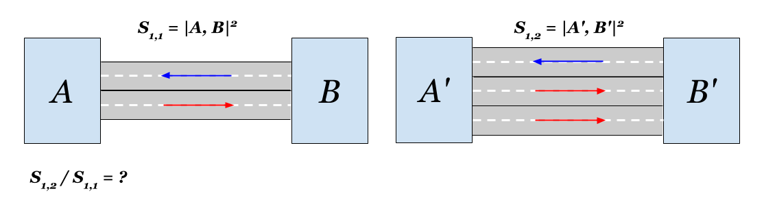
We calculate what is there with our town. If you lay the second lane, the connection in one direction will double. Accordingly, the new distance S1,2(A,B) can be expressed in terms of the source:
S1,2(A,B)=1/ sqrt2cABcBA=1/ sqrt2S1,1(A,B)
The distance between districts will decrease in sqrt2 time. It was obvious, right?
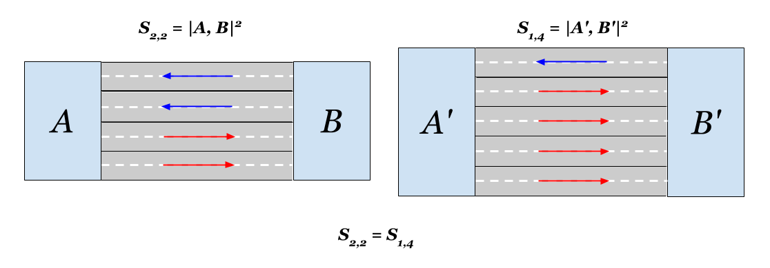
It also turns out that from the point of view of distances, adding one lane to each two-lane road on each side is equivalent to adding three lanes with one. Euclidean proximity in both cases will double. It is interesting.
That's all. Thank you for your attention).
No, not about the mountains - about the graphs. There are questions in mathematics, the wording of which is accessible to everyone, but the solution is nontrivial and difficult to explain without special training. One of the problems of this kind can be briefly expressed in the following way - how can we correctly calculate the distances in directed graphs? This somewhat abstract problem can be reduced to a very specific motivating problem. It fits in one picture:
1. Statement of the problem. I live on one, but you on another.
A small town is divided (for example, by a river, although in the context of the peaks a gorge is more suitable) into two districts (parts) A and B . The communication between the districts is carried out along a single road (bridge), which has two lanes: aside from A to B and back. In connection with the growth of the population, the question arose of increasing the capacity of the road. Money as usual is tight and only enough for one lane in one direction. It is clear that even one lane will bring the regions closer together, but the question is how exactly? You are a
How much closer will the areas be if you build another lane in one direction?
Advanced wording
Instead of
')
And yes, if you are a real
The answer is for those in a hurry
Yes, I was going to give a quick answer here, but changed my mind. Why deprive the reader of the pleasure of independent reflection? Perhaps you offer something more worthwhile than the author. In any case, you can immediately scroll to the end of the article. Sorry).
Measure of closeness and drunkenness
It is clear that the usual (kilometer) distance between the districts does not depend on the presence or absence of the road. Therefore, it will not work here - we need to rely on communication. The more areas are connected - the closer they are, - more residents can get to another area per unit of time.
To estimate the measure of proximity between nodes of an undirected graph, you can use the so-called resistive distance . Earlier we have already described the properties of this distance in several articles in Habré .
Resistive distance is equivalent to the concept of effective resistance when it comes to electrical network. Therefore, in an electric language, the problem can be formulated as follows. Between the two nodes are counter-connected two diodes of equal conductivity. How will the resistance between these points, if you add another diode? (I apologize if I failed the electric language and I wrote nonsense here).
Also, effective resistance can be interpreted in the Markov language of probabilities of
The resistive distance is quadratic, - corresponds to the square of the linear distance. Quadratic distances are also called quadrants . But since other (linear) distances are not used in this problem, we do not need the term quadrant here. (Here and without it there is enough bird language).
In general, the term "resistive distance" also does not look good. He implies that we are talking about some unusual distance unknown to science. In fact, the resistive distance is the usual Euclidean distance . But in affine space. We use this feature of it further.
And what is the problem?
If we know what a “resistive distance” is, then why can't we “just take it and count it” for a given graph?
Hm Basically easy. If we are talking about a non-directed graph. If the city had built lanes in both directions, then the resistive distance would have decreased exactly by half. Since the resistance is inversely proportional to the conductivity, and the conductivity (throughput) doubled. And if I had added two lanes in each direction, then the distance would have decreased by 3 times. It's all quite trivial. (And probably, someone here can already guess about the general form of the solution. And we are going further).
When the counter links are not equal, then everything becomes more complicated. And quite severely.
There is no simplelegalgenerally accepted method for determining the proximity of vertices (resistive distances) in a directed graph .
(This is my thesis - maybe someone can convince me). “No” - here it means that it is not in textbooks, wikis, and in heads (more precisely, there are many different ways from different authors that require different assumptions and definitions). The very way there is (although not so simple). In this article, we just describe it.
The very definition of distance in the presence of directional connections requires clarification if we are talking about a directed graph (noncommutative metric, I apologize). You can talk about the distance from A before B , and you can from B before A . And most likely these distances are not always equal. What kind of distances are we talking about in the problem?
Euclidean distance taxis
Come up and take a deep breath. We have already mentioned that the resistive distance is the usual Euclidean. This means that its definition can be reduced to the definition of the Euclidean distance as the norm of the difference of two elements:
S(A,B)=|A−B|2=(A−B)2=(A−B) cdot(A−B)=S(B,A) quad(1)
This definition does not depend on the order of the elements - it is a commutative distance, proximity (more precisely, the range) of the elements. The point in the expression denotes the operation of the scalar product (the space is metric). Accordingly, the expression (1) can be expanded:
S(A,B)=S(B,A)=A2+B2−A cdotB−B cdotA quad(2)
Here A2=A cdotA , B2=B cdotB - norms of elements. When it comes to graphs, the norms of the elements are usually zero. In the original problem about the norms, nothing is said, so you can take them as zero (in more detail about what the norms of the elements in affine space mean here . And if in more detail, then here ). Then the expression for the desired distance takes the form:
S(A,B)=−(A cdotB+B cdotA)=sAB+sBA quad(3)
According to expression (3), all that is needed to solve a problem is to find the scalar products of elements (nodes) in a directed graph (it is easy to say, but how to do it?).
Along the way, formula (3) shows that our common (commutative) measure of proximity between elements A and B is the sum of two directional distances:
sAB=−A cdotB - directional distance from A before B ,
sBA=−B cdotA - directional distance from B before A .
2. Solution. Long road in the dunes
The general course of reasoning is as follows. We will accurately and without
Any connected graph (whether directed or not) defines an affine metric space. Some properties of such spaces in a symmetric (commutative) design were (chaotic) described in the aforementioned series of articles or more accurately and in detail in the aforementioned longride . Do not rush to switch - we give below (albeit, a patter) basic extracts.
Affine metric space (undirected graph)
What is important. First, the well-known.
1. The affinity of space means that the concepts of vector and element in space are different. The vector is the difference of the elements. This seemingly irrelevant feature leads to significant consequences if a metric is defined in space.
2. The space is given by a basis consisting of elements. The vertices of the graph is the basis of the space. Links in the graph determine its metric properties.
3. The connectivity characteristic of the graph is the adjacency matrix . But for metric (and other) properties, the Laplacian of the graph is more important (Kirchhoff matrix) L .
4. The Laplacian graph is an almost metric tensor. “Almost” - here it means that it is incomplete. Laplacian is a degenerate matrix and therefore not reversible. And the standard metric tensor is completely reversible.
Now less known.
5. The difference between elements and vectors in a metric affine space leads to the existence of a null vector in it. mathbbz . The scalar product of elements with a null-vector in a commutative (symmetric) space is equal to one (in a non-commutative one it depends on the direction of multiplication). Without a null vector, the space of the graph is not complete! It is important.
6. The orthogonal center of the basis is dual with respect to the null-vector. Z . This is an element that is orthogonal to all other elements of the basis (except for the zero vector). Recall that the orthogonality of elements means that their scalar product is zero. The orthocenter of the triangle is the circumcircle . Yes, in a complete affine space, an element with a nonzero norm is not a point, but an n-dimensional sphere.
7. The Laplacian of the graph, together with the coordinates of the orthogonal center, becomes complete (a full metric tensor). In other words, the complete Laplacian Lm - this is the usual laplacian graph L but bordered by the barycentric coordinates of the orthogonal center.
8. Converting a complete Laplacian allows you to get a full Gramian Gm - matrix of scalar products of elements of the basis (in our case, the vertices of the graph). This Gramian is also a full-fledged metric tensor of space.
9. The bordering of the full gramman is a tuple of units (scalar products of the elements of a basis and a zero vector). In the corner - zero, this is the norm of the zero vector itself.
The famous Cayley-Menger matrix is an almost regular Gramian.
As a result, we arrive at the fact that, according to Clause 8, the task of determining scalar products (and, therefore, distances) between nodes of a graph is reduced to the definition of the initial metric tensor of the basis Gm .
We need a method for constructing a complete graph gram. Gm for a given (incomplete) Laplacian L .
In the case of symmetric relations, the construction of a complete Gramian for Laplacian (and vice versa) does not cause any particular difficulties. In this case, the scalar products of the elements of the basis and the zero-vector are commutative - they do not depend on the order of multiplication:
mathbbz cdotA=A cdot mathbbz=1
For directed graphs (noncommutative spaces) the problem becomes more complicated. If only because the number of possible connections in the directed graph is doubled.
Noncommutative affine space (directed graph)
About the properties of the Laplacian directional graph, we also already wrote on Habré . They told how the potentials of the Laplacian can be used to rank objects. In terms of bases, the potentials of the Laplacian are the dual coordinates of the zero vector (the Laplacian annihilator).
In this article, we are interested in metric properties. If the graph is directed, the scalar product between its vertices depends on the order:
A cdotB neB cdotA
This means that the dual coordinates in directed graphs are split (into left and right). The values of the scalar products of the zero-vector and elements of the basis (bordering of the Gramian) also depend on the order of the factors. And therefore, unlike the commutative space, here one half of the dual coordinates of the zero vector is unknown and must be determined.
mathbbz cdotA neA cdot mathbbz
However, there are too many known quantities.
First, the Laplacian itself is known. In addition, it is known that the sum of its rows is zero (in the general case this is an optional requirement, but for the Laplacians of directed graphs this is usually the case). It is also important that the barycentric coordinates of the elements are unique, since they do not depend on the metric of space. That is, the bordering of the laplacian of the graph is symmetrical for both the directional and the undirected graph (I did not immediately recognize this point). Finally, we know the norms of the elements of the basis (usually in graphs they are equal to zero).
It remains to substitute all known and unknown in the identity linking the Laplacian and the Gramians:
Lm Gm=I
Here I - this is the identity matrix. In this identity, the meaning of the transition from an incomplete Laplacian to a complete one.
Shut up and believe
Let's move from words to deeds. This is what the Laplacian looks like. L for a graph of two nodes:
L = \ begin {bmatrix} c_1 & -c_1 \\ c_2 & -c_2 \ end {bmatrix}L = \ begin {bmatrix} c_1 & -c_1 \\ c_2 & -c_2 \ end {bmatrix}
For simplicity, we denote the connection numbers: c1=cAB,c2=cBA . It is assumed that the values of relations are known - through them we will express all the other quantities.
Full laplacian Lm includes orthocenter coordinates [rz,az,bz] :
Lm = \ begin {bmatrix} rz & az & bz \\ az & c_1 & -c_1 \\ bz & c_2 & -c_2 \ end {bmatrix}Lm = \ begin {bmatrix} rz & az & bz \\ az & c_1 & -c_1 \\ bz & c_2 & -c_2 \ end {bmatrix}
Here rz - norm of the orthocenter (in the symmetric case is interpreted as the square of the radius), az and bz - coefficients of decomposition of the orthocenter on the basis A,B (barycentric weights).
Full grammian Gm looks like this:
Gm = \ begin {bmatrix} 0 & za & zb \\ 1 & 0 & g_1 \\ 1 & g_2 & 0 \ end {bmatrix}Gm = \ begin {bmatrix} 0 & za & zb \\ 1 & 0 & g_1 \\ 1 & g_2 & 0 \ end {bmatrix}
Here are tuples [za,zb] and [1,1] reflect the dual coordinates of the null vector. These coordinates are the Laplacian annihilators (when multiplied by the Laplacian, they give a zero vector - not to be confused with a null vector!).
To solve the problem, we need to find the sum of the Gramian values: −(g1+g2) .
We count the number of unknowns: rz,az,bz,za,zb,g1,g2 - only 7 (yes, - to find out the value of one unfortunate distance, we need to calculate another seven additional values). At the entrance there are two known connections - c1 and c2 . Identity Lm Gm=I will give 9 equations. Total 7 + 2 = 9, - everything converges (surprisingly). It remains to simply solve the system of equations.
For a two-node graph, the solution (all unknowns) can be expressed explicitly. We present the final expressions for the quantities of interest to us. We introduce the concept of a common geometric connection - it is the reciprocal of the norm of the orthogonal center. gc=1/rz . Its dimension coincides with the dimension of the connections of the graph. For a graph of two nodes (and two links), the geometric connectivity has a nice expression:
gc=1/rz=( sqrtc1+ sqrtc2)2
Through this connectivity, scalar products of nodes can be expressed:
g1=−gc sqrtc2, quadg2=−gc sqrtc1
You can translate scalar products g in directional distances s (3):
sBA=gc sqrtcAB; quadsBA=gc sqrtcAB
The desired commutative distance between nodes is determined by the sum:
S(A,B)=sBA+sAB=1/ sqrtcABcBA quad(4)
Grandmother arrived
Finally. Expression (4) is the desired formula.
The distance between the vertices of a graph of two nodes is inversely proportional to the square root of the product of counterpropagating connections.
You can load the school textbook with another useless formula.
If the connections are equal, then the result coincides with the resistive distance in non-directional graphs:
Sc,c(A,B)=1/c quad(4.1)
We calculate what is there with our town. If you lay the second lane, the connection in one direction will double. Accordingly, the new distance S1,2(A,B) can be expressed in terms of the source:
S1,2(A,B)=1/ sqrt2cABcBA=1/ sqrt2S1,1(A,B)
The distance between districts will decrease in sqrt2 time. It was obvious, right?
It also turns out that from the point of view of distances, adding one lane to each two-lane road on each side is equivalent to adding three lanes with one. Euclidean proximity in both cases will double. It is interesting.
That's all. Thank you for your attention).
Application. Explicit expressions for the remaining elements of the matrices of our graph
Coordinates of the orthocenter:
az= sqrtc1gc, quadbz sqrtc2gc
Scalar products of basis and null-vector (annihilator of Laplacian):
za= sqrtc2/c1 quadzb= sqrtc1/c2
az= sqrtc1gc, quadbz sqrtc2gc
Scalar products of basis and null-vector (annihilator of Laplacian):
za= sqrtc2/c1 quadzb= sqrtc1/c2
Source: https://habr.com/ru/post/448120/
All Articles