Chaos Information Entropy

Introduction

There are a lot of publications on Habr in which the concept of entropy is considered, these are just some of them [1 ÷ 5]. The publications were positively perceived by the readers and aroused great interest. It is enough to give the definition of entropy given by the author of the publication [1]: “entropy is how much information you do not know about the system”. Publications about the phenomenon of chaos on Habr is also sufficient [6 ÷ 9]. However, the relationship of entropy and chaos in both groups of publications was not considered.

This results from the fact that various areas of knowledge allocate different types of a measure of chaos:
')

informational;
thermodynamic;
differential;
cultural.

It also describes the measures of chaos, taking into account their specificity, even in one of these areas is quite difficult.

Trying to simplify the problem to the utmost, I decided to consider the relationship between informational entropy and chaos on the example of the similarity of the transmission areas from order to chaos on diagrams in the form of point mappings and on graphs of the entropy coefficient for these areas.

What came out of this you will learn by looking under the cat.

Mechanisms of transition from order to chaos

An analysis of the mechanisms of transition from order to chaos in real systems and various models revealed the universality of relatively few transition scenarios to chaos. The transition to chaos can be represented in the form of a diagram of bifurcations (the term “bifurcation” is used to denote the qualitative rearrangements of the system with the emergence of a new mode of its behavior).

The entry of the system into an unpredictable mode is described by a cascade of bifurcations, one after the other. The cascade of bifurcations leads consistently to the appearance of a choice between two solutions, then four, and so on, the system begins to oscillate in a chaotic, turbulent mode of successive doubling of the number of possible values.

We will consider period-doubling bifurcations and the appearance of chaos in point mappings. The display is a function that shows the dependence of the subsequent values of the system parameters on the previous values:

$x_ {n + 1} = f (x_ {n}) = \ lambda x_ {n} (1-x_ {n})$

Consider also the second frequently used function:

$x_ {n + 1} = f (x_ {n}) = \ lambda \ cdot x_ {n} \ cdot (1-x_ {n} ^ {2})$

With the help of point mappings, objects are studied not with continuous but with discrete time . In the transition to the mapping, the dimension of the system under study may decrease.

When the external parameter \ lambda changes, point mappings exhibit a rather complex behavior, which becomes chaotic with sufficiently large \ lambda. Chaos is a very fast running away of trajectories in phase space.

Bifurcation is a qualitative restructuring of the motion picture. The values of the control parameter at which bifurcations occur are called critical or bifurcation values.

To construct the diagrams, we will use the following two listings:

№1. For function:

$x_ {n + 1} = f (x_ {n}) = \ lambda x_ {n} (1-x_ {n})$

Program listing

# -*- coding: utf8 -*- import matplotlib.pyplot as plt from numpy import * def f(a,x0): x1=(a-1)/a#     def ff(x):#  return a*x*(1-x) def fl(x): return x x=x0;y=0;Y=[];X=[] for i in arange(1,1000,1): X.append(x) Y.append(y) y=ff(x) X.append(x) Y.append(y) x=y plt.title('   \n\ $x_{n+1}=\lambda \cdot x_{n}\cdot (1-x_{n})$  $\lambda$ =%s  x0=%s '%(a,x0)) plt.plot(X,Y,'r') x1=arange(0,1,0.001) y1=[ff(x) for x in x1] y2=[fl(x) for x in x1] plt.plot(x1,y1,'b') plt.plot(x1,y2,'g') plt.grid(True) plt.show()

No. 2. For function

$x_ {n + 1} = f (x_ {n}) = \ lambda \ cdot x_ {n} \ cdot (1-x_ {n} ^ {2})$

Program listing

 # -*- coding: utf8 -*- import matplotlib.pyplot as plt from numpy import * def f(a,x0): x1=((a-1)/a)**0.5 def ff(x):#  return a*x*(1-x**2) def fl(x): return x x=x0;y=0;Y=[];X=[] for i in arange(1,1000,1): X.append(x) Y.append(y) y=ff(x) X.append(x) Y.append(y) x=y plt.title('   \n\ $x_{n+1}=\lambda \cdot x_{n}\cdot (1-x_{n}^{2})$  $\lambda$ =%s  x0=%s '%(a,x0)) plt.plot(X,Y,'r') x1=arange(0,1,0.001) y1=[ff(x) for x in x1] y2=[fl(x) for x in x1] plt.plot(x1,y1,'b') plt.plot(x1,y2,'g') plt.grid(True) plt.show()

To assess the impact of the nature of the logistics function on critical values

$\ lambda$ consider diagrams with a function

$x_ {n + 1} = f (x_ {n}) = \ lambda x_ {n} (1-x_ {n})$ for this we will apply listing 1:

When 0 <\ lambda <1 for

$\ lambda = $ 0.9$ and x0 = 0.47 we get the diagram:

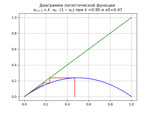
In this case, the mapping has a single fixed point.

$x ^ {*} = 0$
which is sustainable.

With

$1 <\ lambda <3$ for

$\ lambda = 2,5$ x0 = 0.7 we get the diagram:

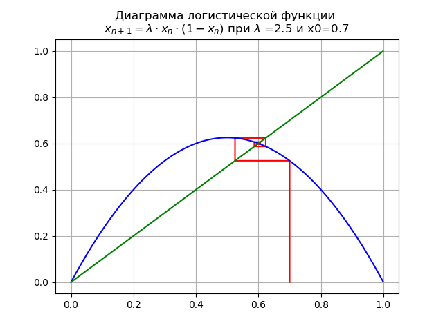
On the interval [0, 1] there appears one more fixed stable point.

$x_ {1} ^ {*} = 1-1 / \ lambda$

With

$1 <\ lambda <3$ for

$\ lambda = 2,5$ and x0 = 0.01 we get the diagram:

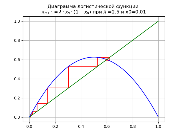
Fixed point

$x ^ {*} = 0$ , loses stability.

With

$3 <\ lambda <3.45$ for

$\ lambda = $ 3.4$ and x0 = 0.7 we get the diagram:

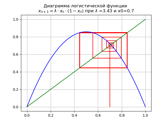
The mapping undergoes bifurcation: fixed point

$x_ {1} ^ {*}$ becomes unstable, and a double cycle appears instead.

With

$3.45 <\ lambda <4.0$ for

$\ lambda = $ 3.5$
and x0 = 0,2 we get the diagram:

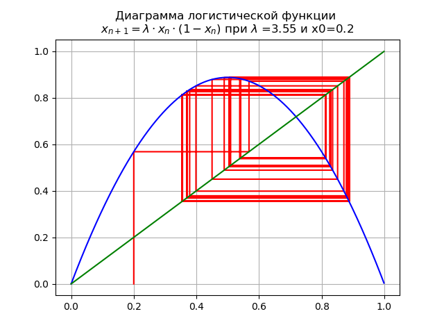
When the transition parameter

$\ lambda$ through value

$\ lambda = 3.45$ The 2-fold cycle becomes 4-fold, and beyond.

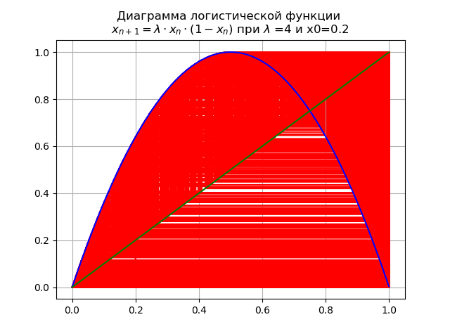
When the final value

$\ lambda = 4$ the system has unstable cycles of all possible orders:

To assess the impact of the nature of the logistics function on critical values

$\ lambda$ consider diagrams with a function

$x_ {n + 1} = f (x_ {n}) = \ lambda \ cdot x_ {n} \ cdot (1-x_ {n} ^ {2})$ For this we will apply listing №2.

With

$0 <\ lambda <= 1.0$ for

$\ lambda = 0.5$ and x0 = 0.2:

The display has a single fixed point.

$x ^ {*} = 0$ which is sustainable.

With

$1 <\ lambda <= 1.998 ...$ for

$\ lambda = 1.8$ and x0 = 0.55:

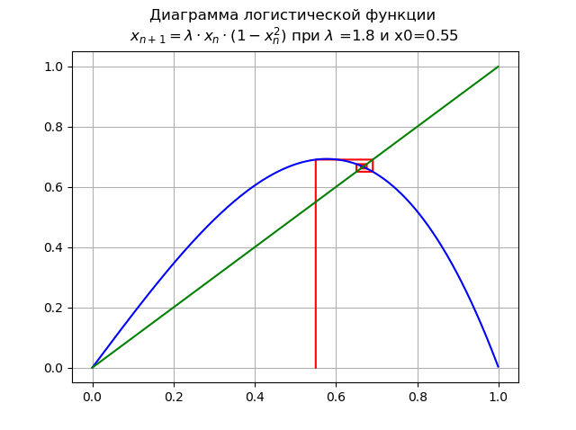
Point

$x ^ {*} = 0$ loses stability, a new stable point appears

$x_ {1} ^ {*}$

With

$1.99 <\ lambda <= 2,235 ...$ for

$\ lambda = 2,2$ and x0 = 0.2:

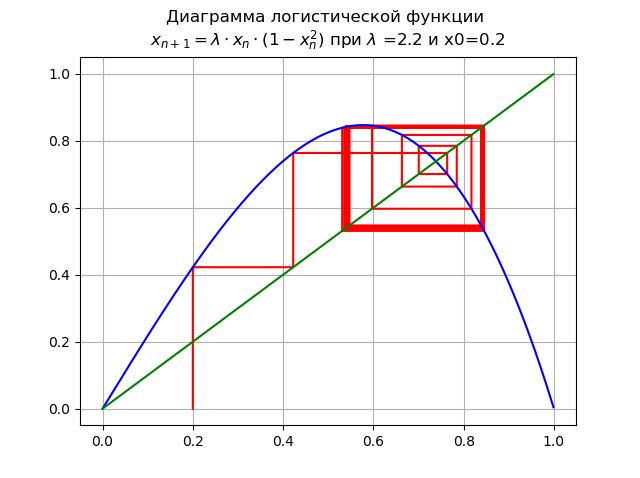
A period doubling bifurcation occurs, a 2-fold cycle appears. Further increase

$\ lambda$ leads to a cascade of period doubling bifurcations.

With

$2,235 <\ lambda 2.5980 ...$ for

$\ lambda = $ 2.28$ and x0 = 0.2:

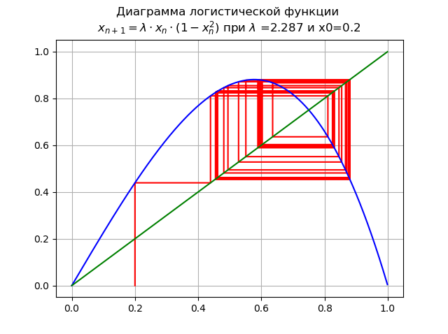
Increase

$\ lambda$ led to a cascade of period-doubling bifurcations.

With

$\ lambda = 2.59$ the system has unstable cycles of all possible periods:

As shown in the diagrams, with increasing order of the logistic function, the range of change

$\ lambda$ tapers off.

Using diagrams, we traced the path from order to chaos, while setting the values

$\ lambda$ for different logistic functions. It remains to answer the question: how to measure chaos? The answer for some of the types of chaos listed at the beginning of this article is known
- entropy measure of chaos. This answer can be fully attributed to informational chaos, however what is the entropy to apply here and how to compare with the already considered numerical value

$\ lambda$ - I will try to answer this question in the next part of the article.

Informational entropy and entropy coefficient

We will consider information binary entropy for independent random events.

$x$ c

$n$ possible states distributed with probabilities

$p_ {i} (i = 1, .., n)$ . Information binary entropy is calculated by the formula:

$H (x) = - \ sum_ {i = 1} ^ {n} p_ {i} \ cdot log_ {2} (p_ {i})$

This value is also called the average message entropy. Magnitude

$H_ {i} = - log_ {2} (p_ {i})$ is called private entropy, which characterizes only the i -e state. In the general case, the base of the logarithm in the definition of entropy can be any greater than 1; his choice determines the unit of measurement of entropy.

We will use decimal logarithms in which entropy and information are measured in bits. The amount of information in bits will be calculated correctly when, for example, variables

$X$ and

$\ Delta$ they will be substituted into the corresponding expressions for entropy no matter what, but necessarily in the same units. Really:

$q = H (x) -H (\ Delta) = log_ {10} \ left (X_ {2} -X_ {1} \ right) -log_ {10} (2 \ Delta) = log_ {10} (\ frac {X_ {2} -X_ {1}} {2 \ Delta})$

where X and

$\ Delta$ must be in the same units.

The estimate of the entropy value of a random variable from experimental data is found by a histogram of the following relationship:

$\ Delta_ {e} = \ frac {1} {2} e ^ {H (x)} = \ frac {d} {2} \ prod_ {i = 1} ^ {m} (\ frac {n} { n_ {i}}) ^ {\ frac {n_ {i}} {n}} = \ frac {dn} {2} 10 ^ {- \ frac {1} {n}} \ sum_ {i = 1} ^ {m} n_ {i} log_ {10} (n_ {i})$

Where:

$d$ –The width of each column of the histogram;

$m$ - number of columns;

$n$ - total amount of data;

$n_ {i}$ - amount of data in

$i$ -that column.

The entropy coefficient is determined from the relationship:

$k_ {e} = \ frac {\ Delta_ {e}} {\ sigma}$

Where:

$\ sigma$ - standard deviation.

Informational entropy as a measure of chaos

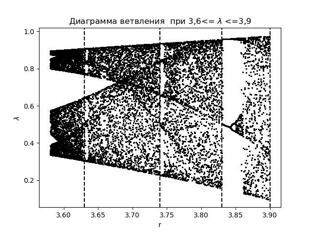
To analyze the phenomena of informational chaos using the entropy coefficient, we first create a branch diagram for the function

$x_ {n + 1} = f (x_ {n}) = \ lambda x_ {n} (1-x_ {n})$ with the application of transition regions obtained in the construction of histograms:

Branch Chart

 import matplotlib.pyplot as plt import matplotlib.pyplot as plt from numpy import* N=1000 y=[] y.append(0.5) for r in arange(3.58,3.9,0.0001): for n in arange(1,N,1): y.append(round(r*y[n-1]*(1-y[n-1]),4)) y=y[N-250:N] x=[r ]*250 plt.plot( x,y, color='black', linestyle=' ', marker='.', markersize=1) plt.figure(1) plt.title("   3,6<= $\lambda$ <=3,9") plt.xlabel("r") plt.ylabel("$\lambda$ ") plt.axvline(x=3.63,color='black',linestyle='--') plt.axvline(x=3.74,color='black',linestyle='--') plt.axvline(x=3.83,color='black',linestyle='--') plt.axvline(x=3.9,color='black',linestyle='--') plt.show()

We get:

Construct a graph for the entropy coefficient for the same areas

$\ lambda$ :

Graph for entropy coefficient

 import matplotlib.pyplot as plt from numpy import* data_k=[] m='auto' for p in arange(3.58,3.9,0.0001): q=[round(p,2)] M=zeros([1001,1]) for j in arange(0,1,1): M[0,j]=0.5 for j in arange(0,1,1): for i in arange(1,1001,1): M[i,j]=q[j]*M[i-1,j]*(1-M[i-1,j]) a=[] for i in arange(0,1001,1): a.append(M[i,0]) n=len(a) z=histogram(a, bins=m) if type(m) is str: m=len(z[0]) y=z[0] d=z[1][1]-z[1][0] h=0.5*d*n*10**(-sum([w*log10(w) for w in y if w!=0])/n) ke=round(h/std(a),3) data_k.append(ke) plt.title("  ke  3,6<= $\lambda$ <=3,9") plt.plot(arange(3.58,3.9,0.0001),data_k) plt.xlabel("$\lambda$ ") plt.ylabel("ke") plt.axvline(x=3.63,color='black',linestyle='--') plt.axvline(x=3.74,color='black',linestyle='--') plt.axvline(x=3.83,color='black',linestyle='--') plt.axvline(x=3.9,color='black',linestyle='--') plt.grid() plt.show()

We get:

Comparing the diagram and the graph, we see an identical display of the regions in the diagram and in the graph for the entropy coefficient for the function

$x_ {n + 1} = f (x_ {n}) = \ lambda x_ {n} (1-x_ {n})$ .

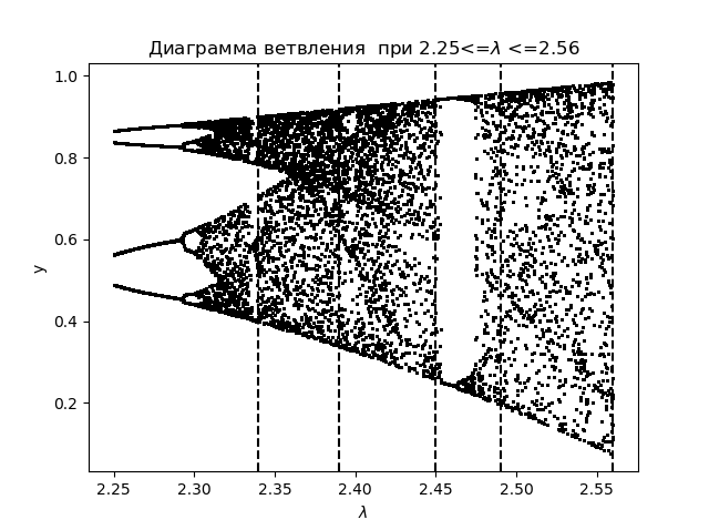
For further analysis of the phenomena of information chaos using the entropy coefficient, we will create a branch diagram for the logistic function:

$x_ {n + 1} = f (x_ {n}) = \ lambda \ cdot x_ {n} \ cdot (1-x_ {n} ^ {2})$ with the application of transition areas:

Branch Chart

 import matplotlib.pyplot as plt from numpy import* N=1000 y=[] y.append(0.5) for r in arange(2.25,2.56,0.0001): for n in arange(1,N,1): y.append(round(r*y[n-1]*(1-(y[n-1])**2),4)) y=y[N-250:N] x=[r ]*250 plt.plot( x,y, color='black', linestyle=' ', marker='.', markersize=1) plt.figure(1) plt.title("   2.25<=$\lambda$ <=2.56") plt.xlabel("$\lambda$ ") plt.ylabel("y") plt.axvline(x=2.34,color='black',linestyle='--') plt.axvline(x=2.39,color='black',linestyle='--') plt.axvline(x=2.45,color='black',linestyle='--') plt.axvline(x=2.49,color='black',linestyle='--') plt.axvline(x=2.56,color='black',linestyle='--') plt.show()

We get:

Construct a graph for the entropy coefficient for the same areas

$\ lambda$ :

Entropy Ratio Graph

 import matplotlib.pyplot as plt from numpy import* data_k=[] m='auto' for p in arange(2.25,2.56,0.0001): q=[round(p,2)] M=zeros([1001,1]) for j in arange(0,1,1): M[0,j]=0.5 for j in arange(0,1,1): for i in arange(1,1001,1): M[i,j]=q[j]*M[i-1,j]*(1-(M[i-1,j])**2) a=[] for i in arange(0,1001,1): a.append(M[i,0]) n=len(a) z=histogram(a, bins=m) if type(m) is str: m=len(z[0]) y=z[0] d=z[1][1]-z[1][0] h=0.5*d*n*10**(-sum([w*log10(w) for w in y if w!=0])/n) ke=round(h/std(a),3) data_k.append(ke) plt.figure(2) plt.title("  ke  2.25<= $\lambda$ <=2.56") plt.plot(arange(2.25,2.56,0.0001),data_k) plt.xlabel("$\lambda$ ") plt.ylabel("ke") plt.axvline(x=2.34,color='black',linestyle='--') plt.axvline(x=2.39,color='black',linestyle='--') plt.axvline(x=2.45,color='black',linestyle='--') plt.axvline(x=2.49,color='black',linestyle='--') plt.axvline(x=2.56,color='black',linestyle='--') plt.grid() plt.show()

We get:

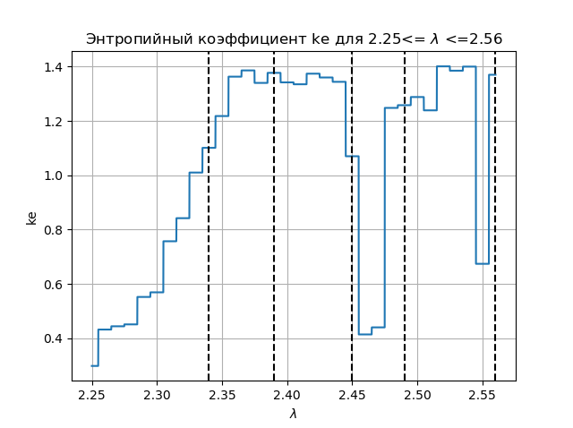
Comparing the diagram and the graph, we see an identical display of the regions in the diagram and in the graph for the entropy coefficient for the function

$x_ {n + 1} = f (x_ {n}) = \ lambda \ cdot x_ {n} \ cdot (1-x_ {n} ^ {2})$

Findings:

The article solved the educational problem: is the informational entropy a measure of chaos, and the means of Python are given an affirmative answer to this question.

Links

Source: https://habr.com/ru/post/447874/

All Articles

Chaos Information Entropy

Introduction

Mechanisms of transition from order to chaos

Informational entropy and entropy coefficient

Informational entropy as a measure of chaos

Findings:

Links

More articles: