Foreword

I think we need to briefly explain why suddenly such a seemingly trivial topic with the calculation of the energy budget and why exactly the CubeSat satellites? Well, everything is quite simple here: my short pedagogical practice has shown (to me) that this topic, although basic, is far from being understood by everyone from the first time, and moreover, it has several unobvious questions in the first reading. Moreover, it would seem that such basic things still publish articles in IEEE and are far from being made by students . Why CubeSat? It is still simpler here: the satellite format is interesting (the very fact of the existence of micro- and nanosatellites, as it turned out, plunges many into a state of short shock), and therefore it is not suitable for educational purposes by the way.

The simulation will be conducted in python 3 for the same reasons that I expressed in my previous publication . We will consider the low-orbit case (LEO - Low Earth Orbit), and calculate, in fact, the signal-to-noise ratio (SNR - Signal-to-Noise ratio) at the receiver input on the downlink (DL - Down Link). We will use several directories from open access and build graphs for clarity.

All source codes are available in my GitHub repository , I invite everyone interested to read! For the code review and constructive criticism I will be very grateful!

Go!

What formulas will we calculate?

First, of course, everyone (involved in the subject) has a well-known formula for the signal-to-noise ratio on a logarithmic scale (in decibels, in a simple way), where we take all possible losses and amplifications with a certain degree of abstraction:

Where - total thermal noise power (related to spectral noise density ) in dBm (decibel per milivatt), - transmit power in dBm, and - antenna gains on the transmitter and receiver side, respectively (in dBi - isotropic decibels), and - transmitter and receiver feeder gain (in dB), and - feeder loss (in dB), losses in the propagation of an electromagnetic wave in dB, - additional losses (some kind of margin (so to speak) in dB).

In general, with the first seven items everything is more or less clear: the data are for reference. More interesting is the situation with the last three participants in the process.

Thermal noise power

As you know, there is nowhere to hide from this scourge of electronic devices, you can only take into account:

Where - Boltzmann constant, - equivalent noise temperature, - the sum of the loss of the antenna and the noise (background) of the sky, - receiver noise temperature ( , but - noise figure, which can be estimated from the noise picture ( - noise figure) receiving antenna), and - the width of the frequency band noise. You can take the noise band equal to the bandwidth of the receiver itself However, according to [1, p.98] the noise bandwidth can be rated a little more accurately as where - constant from 1.002 to 1.57 (refers to the configuration of the receiver).

Additional loss

Here you can either accept some kind of guaranteed stock, drawn, as a rule, from the same reference books, or go deeper and calculate everything yourself.

In this section, I almost completely rely on the good old Kantor textbook, namely on this part of it [1, p.88-96]. If readers have more relevant authoritative sources - please share, I think it will be useful to everyone.

First of all, pay attention to:

1. Losses due to refraction and inaccurate antenna pointing ( Antenna Beam Loss )

Denoted as where - beam width and - beam width of half power, and depend, no matter how hard to guess, on the characteristics of certain antenna devices:

1. Phase effects in the atmosphere

If you believe the classics, then these losses primarily affect the data transfer rate due to the receiver bandwidth, since the band should be chosen in accordance with Table 1 [1, p. 91]. To avoid phase distortion.

Tab. 1. Maximum receiver bandwidth for different ranges.

Although, it should be noted that the numbers are very impressive and often not considered, rather, due to thermal noise.

1. Losses due to inconsistency of antenna polarization

It can be estimated depending on the ellipticity coefficients. $$$e_1$and $$$e_2$(I attach a clipping from the Soviet book as Figure 1).

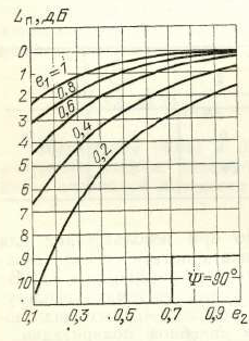
Fig.1. Dependence of losses due to inconsistency of the polarizations of the transmitting and receiving antennas on ellipticity. [1, p. 93]

However, I came across this parameter as reference data. For example, in the calculation of the energy budget for the NanoCom AX100, the polarization loss is 3 dB (atmospheric loss is 2.1 dB, ionospheric loss is 0.4 dB).

1. Atmospheric attenuation

We can estimate this interesting parameter either according to ITU recommendations , or calculate it yourself. Fortunately, there are special libraries like this .

Attenuation in the propagation path of an electromagnetic wave (Path Loss)

Without further ado, let's apply the Phrytic formula to start :

Where - electromagnetic wavelength (refers in a known manner to the carrier frequency , - the speed of an electromagnetic wave (the speed of light, if simpler)), and - the distance between the satellites and the ground station.

And here we come, perhaps, to the most interesting question: what is the distance to take for calculations? As already mentioned in the introduction, we are considering LEO satellites, which means that relative to the Earth our intended satellite is moving (unlike the geostationary case in which the satellite, as it were, hangs above one point).

You can, of course, simplify everything as much as possible by taking the scheme as the basis (Fig. 2), when it is assumed that the communications satellite orbit is, roughly speaking, “above the head” of our ground station.

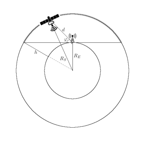
Fig. 2. Schematic description of the CubeSat trajectory in low Earth orbit [2].

Then the distance can be calculated by the formula:

Where - there is, in fact, the radius of the Earth, - the height of the satellite orbit, and - elevation angle.

However, it is possible to steam up a little more, turn again to the classic (to another) [3, p.110-123] and calculate everything already relative to the real geographical coordinates of the ground station (
and ) and the real position of the satellite (instantaneous longitude of the ascending node - instantaneous ascending node and instant orbit poles - instantaneous orbit pole ). Get ready, there will be a lot of trigonometry:

Where - the minimum central angle of the Earth, - the minimum nadir angle - the angular radius of the Earth. The maximum distance can be calculated by:

Where and ( - Minimum satellite elevation angle).

Let's summarize the parameters :

1. What we choose as starting points : the carrier frequency, the height of the orbit (perhaps the position of the satellite and the geographic coordinates of the ground station - depends on the accuracy we want to receive);
2. We find equipment dependent and adjustable parameters : transmitted power, receiver bandwidth;
3. We find reference data : gain and loss of the antenna, gain and loss in the feeder, noise temperature, additional loss.

Let's model what happened in the end

As a source of technical parameters for downlink evaluation, real examples of transceivers and antennas for CubeSat satellites, such as the NanoCom AX100 and NanoCom ANT430, are available to us . For greater bandwidth it is better, of course, to consider the S-band . NanoCom ANT2000 patch antenna and NanoCom SR2000 transceiver are available for this range.

We start to check what happened.

from SmallSatLB import * import pandas as pd 

All logic is conventionally divided into two options: 'draft' , in which the formula (4) is used to calculate the distance; and 'precise' , in which formulas (5) and (6) are used.

'draft'

 l_d = LinkBudget(750*1e3, 'draft') #   (   ) d = l_d.distance() #   phi = np.pi*np.array(range(0,181,5))/180 #     plt.plot(180*phi/np.pi, d*1e-3, '-o') plt.title('Distances') plt.xlabel('Elevation angles (degrees)') plt.ylabel('Distance (km)') plt.grid()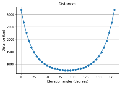 

 snr, EIRP = l_d.expected_snr(2.4e9, 1, 7.3, 35, 1.5e6, 1000) #  SNR plt.title('Expected SNRs') plt.xlabel('Elevation angles (degrees)') plt.ylabel('SNR (dB)') plt.legend() plt.grid() 

Beauty!

'precise'

 l_p = LinkBudget(750*1e3, 'precise',\ L_node = 100+90, incl = 90 - 61.5,\ lat_gs = 22, long_gs = 200, eps_min = 5) snr, EIRP = l_p.expected_snr(2.4e9, 1, 7.3, 35, 1.5e6, 1000) print(min(snr)) print(max(snr)) 

 >>> 5.556823874020452 >>> 8.667000351847676 

In general, here: we have a small tool for initial “estimations” and calculations of how weak the signal is, while it goes from satellite to Earth (or vice versa).
Thank you all for your attention!

References :

1. Kantor L. Ya., Askinazy G. B. Satellite communication and broadcasting: a reference book . - Radio and communication, 1988.
2. Otilia Popescuy, Jason S. Harrisz and Dimitrie C. Popescuz, Designing the Communication Sub-System for Nanoscale Subjects: Operational and Implementation Perspectives, 2016, IEEE
3. Wertz JR, Larson WJ Space Mission Analysis and Space Technology Library. - Microcosm Press and Kluwer Academic Publishers, El Segundo, CA, USA ,, 1999.