On the application of the theory of ARMA-processes in engineering practice
Below we will say a few words about the well-known in general, but most often quite discrete-temporary alternative for engineering workers to mathematical models in the form of linear differential equations, namely, autoregression models - a moving average, and very unusual perspectives of such modeling, the capabilities of which far exceed what used to receive from LDU.
The list of potential capabilities of the technology includes the analysis of systems with an incoming disturbance unavailable for observation, determination of the resonant properties of such systems, the spectrum and the process of external excitation itself, spectral estimation of the processes by their short implementations, modeling the behavior of systems at a low sampling rate over time, etc.

')
ARMA processes, well known to economists (more precisely, “econometricians”), are noticeably less so to specialists in automatic regulation, and, in my opinion, are almost never used by mechanical engineers and radio electronics, especially “old schooling”. The article attempts to indicate some possible areas of application of ARMA theory in engineering practice.
In a nutshell, simplified, for those unfamiliar with the subject, which, in fact, is. For the stochastic continuous-time process x (t) for obvious “digital” reasons, in practice, the discrete-time sequence x [i] is usually associated with the sampling interval Δt.
In principle, for any process x [i] it is possible to represent the form
x [i] - a 1 · x [i-1] - a 2 · x [i-2] - ... - a p · x [ip] = b 0 · f [i] + b 1 · f [i- 1] + ... + b q · f [iq] (1),
where a k and b k are the constant (for this model) coefficients, called the autoregression-moving average model with the order of autoregression p and the moving average q. or ARMA (p, q) -model, f [i] - a kind of "incoming" process, about which just below. Often (1) is written in a slightly different form (6).
In general, this is just a digital filter that has both recursive AR and non-recursive MA parts.
ARMA (p, q) -models conform to linear systems (for example, mechanical), for example, described by the well-known linear differential equation of the form
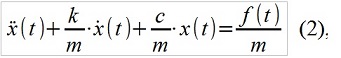
where m, c, k is the mass, stiffness and damping of the mechanical system, f (t) is the external force effect. ARMA-analogue looks like this:
x [i] - a 1 · x [i-1] - a 2 · x [i-2] = b 1 · f [i-1] (3),
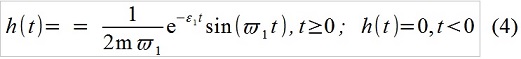
model coefficients can be quite easily found using the eigenvalues λ 1 and λ 1 * (for brevity, the “oscillating” case is considered) of the linear system and Δt:
a 1 = z + z *, a 2 = - z · z *, b 1 = j (z * -z) · Δt / (2mω 1 ),
where z = exp (λ 1 · Δt), λ 1 = -ε 1 + jω 1 , j is the imaginary unit, * is complex conjugation
Reference: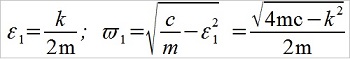
For the test system was taken m = 1 kg, c = 100 N / m, k = 0.75 kg / s, Δt = 0.12 s.,
ARMA (2,1) model obtained
x [i] - 0.69433x [i-1] +0.91393 x [i-2] = 0.010696 · f [i-1]
(A very brief explanation of how (3) generally produces (3). The impulse transition function of our linear system, i.e. the system response to a single impulse:
The record (2) in the "integral" form is called the "convolution" f (t) and h (t), meaning implies consideration of external influence, as a sequence of elementary impulses. In discrete time, write, well, for example, like this:

By adding x [i], x [i-1] and x [i-2] using selected factors 1, a 1 and a 2 achieve mutual destruction of the infinite "tails" h [i] - f [i] remain in the right part · H [0] = f [i] · 0 and f [i-1] · h [1] = f [i-1] · b 1 . From the point of view of the ARMA theory, an infinite-dimensional moving average MA model (∞) was converted into ARMA (2,1) (although some would say that the purely autoregressive model AR (2) = ARMA (2.0) was accidentally obtained).
Remark 1. The reader who knows about the digital processing of processes will say that it is not very correct to sample h (t) just like that - you need to limit the function h (t) in frequency to 1 / (2Δt) (filter out). Otherwise, there is a frequency masking error. In the depicted graphs of the frequency response and phase response of our system, the “analytical” and ARMA model, it is clear why this error can most likely be neglected in most engineering cases (Fig. 1) (here the frequency response is on a logarithmic scale).
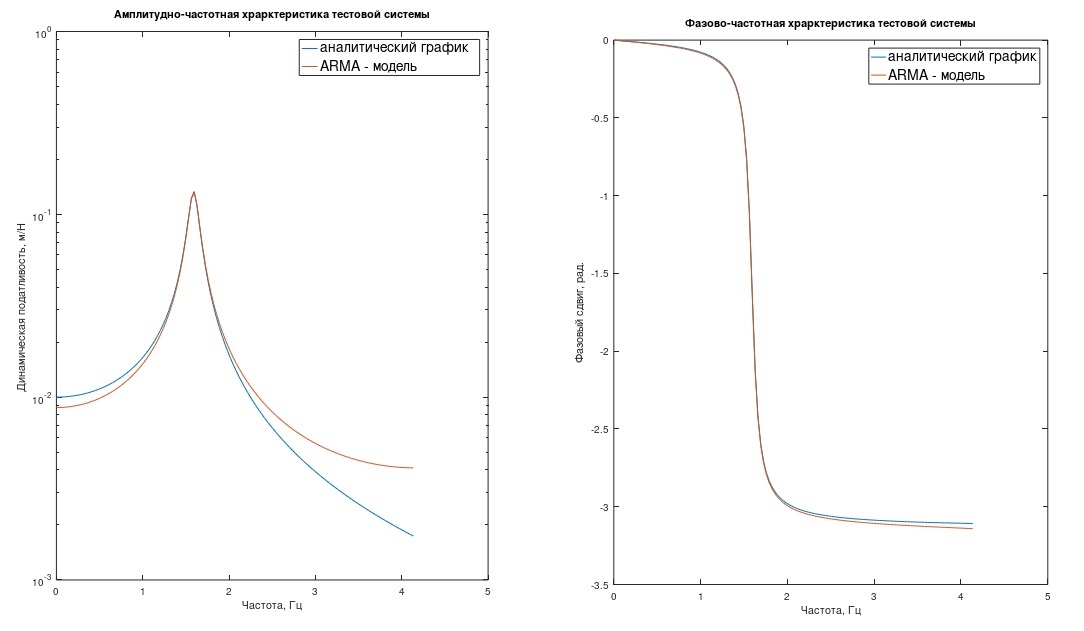
Figure 1 of the frequency response and phase response of the test system.
Remark 2. In practice, the order of the ARMA model can be substantially larger than the example considered above, due to, say, several degrees of freedom of a mechanical system or a complex spectrum of real external influence.
Remark 3. Very important. There are methods (there are not considered here - many more articles can be written about them), allowing to evaluate the parameters of the ARMA model (namely, the order of the model p and q and the coefficients a k and b k ) only by the resulting process x [i], assuming that f [i] is a hypothetical white noise, the variance of which can also be estimated. In general, such an assessment is the main part of the whole ARMA theory. Special perfection while these methods do not differ, but they are of considerable interest.
Now, about why, in fact, all this could (or could) be applied in practice. In addition to the obvious - the quick construction of “manually” damped (and continuous) sinusoids over the first two points and two coefficients a 1 and a 2 , there are, in my opinion, more serious applications of these models in engineering practice.
1. Well, actually, for the simulation modeling of the system operation - we give a real external signal f [i] to the input, we get x [i] at the output:
x [i] = a 1 · x [i-1] + a 2 · x [i-2] +… + a p · x [ip] + b 0 · f [i] + b 1 · f [i- 1] + ... + b q · f [iq] (6)
The ARMA model does the task better than the finite difference model, although it is noticeable only with large sampling intervals Δt. (in Fig. 2, Δt = 0.12 s (left) and 0.03 s). In what cases it makes sense to mess with ARMA - you decide.
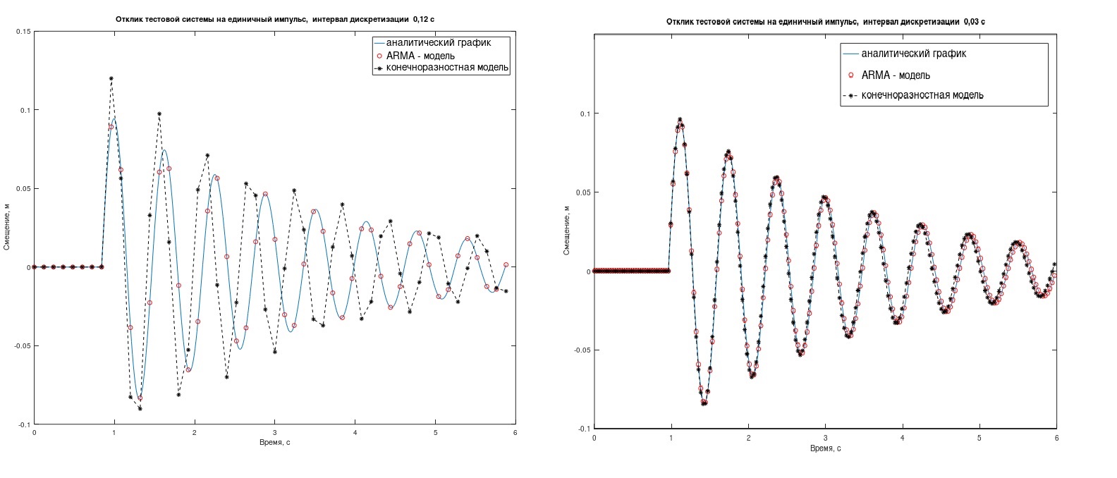
rice 2. The response of test systems to a single impulse.
2. For spectral estimation, especially when there is not enough stationary process available for observation. Perhaps this is the most famous engineering application of ARMA-models. Since for the process being studied both a digital filter and the dispersion of the white noise entering it will be obtained, the problem of constructing an SPM estimate is solved in an obvious way. Indeed, it is possible to get externally very “smooth” graphics of SPM and at the same time creating the impression of high resolution. The expected improvements in the assessment are attributed to the fact that the researcher introduces external information about the nature of the process into the assessment structure — usually by specifying the known order of the model.
In short, you need to know how this SPM should look like. “Exploration” studies of this implementation with the help of classical methods can give little, mainly referring to classical (based on FFT) studies of similar in nature, but significantly longer implementations. There is a possibility of gross errors.
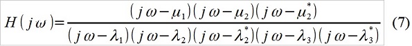
3. To analyze the resonant properties of the system and the spectrum of external influence, in the case when the true external influence is not available for observation. As already noted, it is possible, knowing the process x [i], to determine all the coefficients of the model a k and b k (and the variance of the incoming white noise). Using them, determining the roots of two polynomials with the corresponding coefficients, it is easy to find the p "poles" and q "zeros" of the model (λ k and μ k ) and build its transfer function - you can probably not even in ARMA form (here it is not is given), and in the usual "analytical" form - as we found out above (Fig. 1), the difference is small. For example, for p = 5, q = 3 (while distracting from the existing, apparently, restrictions on the ratio of p and q), alternatively, we have:
All very, very simplistic, of course. Based on the known nature of the object under study (for example, it is a field test of the smoothness of the car) and external influence (road microprofile), the transfer function the researcher decided to rewrite, for example, like this:
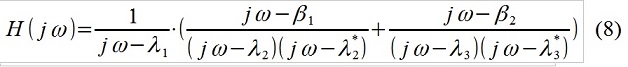
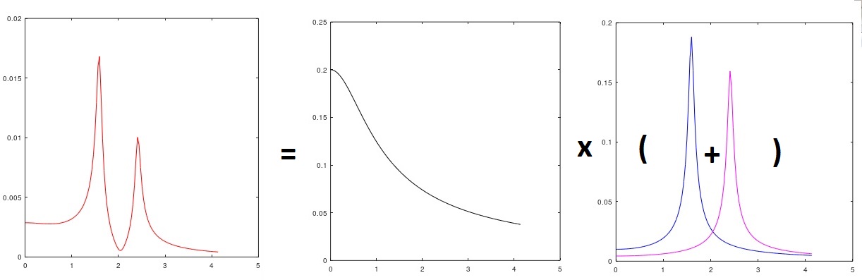
Fig.3. Analysis of the signal spectrum with the selection of the incoming disturbance
and commented - the part of the model associated with λ 1 is, obviously (up to squaring and multiplying by the variance of the incoming hypothetical white noise) the “pink” microprofile of the road (Fig. 3) (i.e., we have identified the unknown spectrum of the real the incoming signal was chosen manually - it seems like “similar”), λ 2 and λ 3 - the resonant properties of the body on the suspension (perhaps, the longitudinal-angular and vertical forms of vibrations). The main problem will be, of course, in determining the parameters of the ARMA-model. For what has just been described, it is sometimes possible without any ARMA to “crawl” (albeit electronically) according to the spectral density graph and measure the width of the peaks at the level of -3 dB, etc., or use curvfitting, sometimes with more success. .
3. For linear prediction, x [i]. Apparently, the main application of ARMA from "econometricians". From (6) it can be seen that if the model's coefficients were able to be assessed using the methods generally mentioned above, the next value of x [i] can be estimated with accuracy up to observable hypothetical white noise b 0 · f [i], the dispersion of this white noise is estimated together with the coefficients of the model. Usually, in this case, a dynamic (real-time) adjustment of model parameters is implied. Apparently, it can be useful in systems of active vibration and noise reduction. TAR specialists know best.
4. To restore an inaccessible incoming process. When the model is divided into parts, as was shown above in section 3, based on knowledge of the nature of the process being studied, it is possible to estimate separately the spectrum of the incoming disturbance, separately - the oscillatory properties of the physical system (divide the model into parts). You can go further - to create a filter (ARMA-model, the inverse of the original model), connecting the system output with the input, and with its help from the resulting process x [i] get the time implementation of the incoming disturbance. For example, try to restore an undistorted signal recorded with exactly unknown linear distortions by equipment that is inaccessible for a separate study (say, obtained by telemetry).
Based on my modest knowledge, in the end I will express such a subjective judgment. The applicability of ARMA technologies to engineering problems strongly depends on the perfection of methods for estimating the parameters of these models from the resulting signal, more precisely, in my opinion, is strongly constrained by the imperfection of these methods. Working out the experience of using ARMA in engineering seems to make sense, mainly on the threshold of a very likely “breakthrough” in this area.
The list of potential capabilities of the technology includes the analysis of systems with an incoming disturbance unavailable for observation, determination of the resonant properties of such systems, the spectrum and the process of external excitation itself, spectral estimation of the processes by their short implementations, modeling the behavior of systems at a low sampling rate over time, etc.
')
ARMA processes, well known to economists (more precisely, “econometricians”), are noticeably less so to specialists in automatic regulation, and, in my opinion, are almost never used by mechanical engineers and radio electronics, especially “old schooling”. The article attempts to indicate some possible areas of application of ARMA theory in engineering practice.
In a nutshell, simplified, for those unfamiliar with the subject, which, in fact, is. For the stochastic continuous-time process x (t) for obvious “digital” reasons, in practice, the discrete-time sequence x [i] is usually associated with the sampling interval Δt.
In principle, for any process x [i] it is possible to represent the form
x [i] - a 1 · x [i-1] - a 2 · x [i-2] - ... - a p · x [ip] = b 0 · f [i] + b 1 · f [i- 1] + ... + b q · f [iq] (1),
where a k and b k are the constant (for this model) coefficients, called the autoregression-moving average model with the order of autoregression p and the moving average q. or ARMA (p, q) -model, f [i] - a kind of "incoming" process, about which just below. Often (1) is written in a slightly different form (6).
In general, this is just a digital filter that has both recursive AR and non-recursive MA parts.
ARMA (p, q) -models conform to linear systems (for example, mechanical), for example, described by the well-known linear differential equation of the form
where m, c, k is the mass, stiffness and damping of the mechanical system, f (t) is the external force effect. ARMA-analogue looks like this:
x [i] - a 1 · x [i-1] - a 2 · x [i-2] = b 1 · f [i-1] (3),
model coefficients can be quite easily found using the eigenvalues λ 1 and λ 1 * (for brevity, the “oscillating” case is considered) of the linear system and Δt:
a 1 = z + z *, a 2 = - z · z *, b 1 = j (z * -z) · Δt / (2mω 1 ),
where z = exp (λ 1 · Δt), λ 1 = -ε 1 + jω 1 , j is the imaginary unit, * is complex conjugation
Reference:
For the test system was taken m = 1 kg, c = 100 N / m, k = 0.75 kg / s, Δt = 0.12 s.,
ARMA (2,1) model obtained
x [i] - 0.69433x [i-1] +0.91393 x [i-2] = 0.010696 · f [i-1]
(A very brief explanation of how (3) generally produces (3). The impulse transition function of our linear system, i.e. the system response to a single impulse:
The record (2) in the "integral" form is called the "convolution" f (t) and h (t), meaning implies consideration of external influence, as a sequence of elementary impulses. In discrete time, write, well, for example, like this:
By adding x [i], x [i-1] and x [i-2] using selected factors 1, a 1 and a 2 achieve mutual destruction of the infinite "tails" h [i] - f [i] remain in the right part · H [0] = f [i] · 0 and f [i-1] · h [1] = f [i-1] · b 1 . From the point of view of the ARMA theory, an infinite-dimensional moving average MA model (∞) was converted into ARMA (2,1) (although some would say that the purely autoregressive model AR (2) = ARMA (2.0) was accidentally obtained).
Remark 1. The reader who knows about the digital processing of processes will say that it is not very correct to sample h (t) just like that - you need to limit the function h (t) in frequency to 1 / (2Δt) (filter out). Otherwise, there is a frequency masking error. In the depicted graphs of the frequency response and phase response of our system, the “analytical” and ARMA model, it is clear why this error can most likely be neglected in most engineering cases (Fig. 1) (here the frequency response is on a logarithmic scale).
Figure 1 of the frequency response and phase response of the test system.
Remark 2. In practice, the order of the ARMA model can be substantially larger than the example considered above, due to, say, several degrees of freedom of a mechanical system or a complex spectrum of real external influence.
Remark 3. Very important. There are methods (there are not considered here - many more articles can be written about them), allowing to evaluate the parameters of the ARMA model (namely, the order of the model p and q and the coefficients a k and b k ) only by the resulting process x [i], assuming that f [i] is a hypothetical white noise, the variance of which can also be estimated. In general, such an assessment is the main part of the whole ARMA theory. Special perfection while these methods do not differ, but they are of considerable interest.
Now, about why, in fact, all this could (or could) be applied in practice. In addition to the obvious - the quick construction of “manually” damped (and continuous) sinusoids over the first two points and two coefficients a 1 and a 2 , there are, in my opinion, more serious applications of these models in engineering practice.
1. Well, actually, for the simulation modeling of the system operation - we give a real external signal f [i] to the input, we get x [i] at the output:
x [i] = a 1 · x [i-1] + a 2 · x [i-2] +… + a p · x [ip] + b 0 · f [i] + b 1 · f [i- 1] + ... + b q · f [iq] (6)
The ARMA model does the task better than the finite difference model, although it is noticeable only with large sampling intervals Δt. (in Fig. 2, Δt = 0.12 s (left) and 0.03 s). In what cases it makes sense to mess with ARMA - you decide.
rice 2. The response of test systems to a single impulse.
2. For spectral estimation, especially when there is not enough stationary process available for observation. Perhaps this is the most famous engineering application of ARMA-models. Since for the process being studied both a digital filter and the dispersion of the white noise entering it will be obtained, the problem of constructing an SPM estimate is solved in an obvious way. Indeed, it is possible to get externally very “smooth” graphics of SPM and at the same time creating the impression of high resolution. The expected improvements in the assessment are attributed to the fact that the researcher introduces external information about the nature of the process into the assessment structure — usually by specifying the known order of the model.
In short, you need to know how this SPM should look like. “Exploration” studies of this implementation with the help of classical methods can give little, mainly referring to classical (based on FFT) studies of similar in nature, but significantly longer implementations. There is a possibility of gross errors.
3. To analyze the resonant properties of the system and the spectrum of external influence, in the case when the true external influence is not available for observation. As already noted, it is possible, knowing the process x [i], to determine all the coefficients of the model a k and b k (and the variance of the incoming white noise). Using them, determining the roots of two polynomials with the corresponding coefficients, it is easy to find the p "poles" and q "zeros" of the model (λ k and μ k ) and build its transfer function - you can probably not even in ARMA form (here it is not is given), and in the usual "analytical" form - as we found out above (Fig. 1), the difference is small. For example, for p = 5, q = 3 (while distracting from the existing, apparently, restrictions on the ratio of p and q), alternatively, we have:
All very, very simplistic, of course. Based on the known nature of the object under study (for example, it is a field test of the smoothness of the car) and external influence (road microprofile), the transfer function the researcher decided to rewrite, for example, like this:
Fig.3. Analysis of the signal spectrum with the selection of the incoming disturbance
and commented - the part of the model associated with λ 1 is, obviously (up to squaring and multiplying by the variance of the incoming hypothetical white noise) the “pink” microprofile of the road (Fig. 3) (i.e., we have identified the unknown spectrum of the real the incoming signal was chosen manually - it seems like “similar”), λ 2 and λ 3 - the resonant properties of the body on the suspension (perhaps, the longitudinal-angular and vertical forms of vibrations). The main problem will be, of course, in determining the parameters of the ARMA-model. For what has just been described, it is sometimes possible without any ARMA to “crawl” (albeit electronically) according to the spectral density graph and measure the width of the peaks at the level of -3 dB, etc., or use curvfitting, sometimes with more success. .
3. For linear prediction, x [i]. Apparently, the main application of ARMA from "econometricians". From (6) it can be seen that if the model's coefficients were able to be assessed using the methods generally mentioned above, the next value of x [i] can be estimated with accuracy up to observable hypothetical white noise b 0 · f [i], the dispersion of this white noise is estimated together with the coefficients of the model. Usually, in this case, a dynamic (real-time) adjustment of model parameters is implied. Apparently, it can be useful in systems of active vibration and noise reduction. TAR specialists know best.
4. To restore an inaccessible incoming process. When the model is divided into parts, as was shown above in section 3, based on knowledge of the nature of the process being studied, it is possible to estimate separately the spectrum of the incoming disturbance, separately - the oscillatory properties of the physical system (divide the model into parts). You can go further - to create a filter (ARMA-model, the inverse of the original model), connecting the system output with the input, and with its help from the resulting process x [i] get the time implementation of the incoming disturbance. For example, try to restore an undistorted signal recorded with exactly unknown linear distortions by equipment that is inaccessible for a separate study (say, obtained by telemetry).
Based on my modest knowledge, in the end I will express such a subjective judgment. The applicability of ARMA technologies to engineering problems strongly depends on the perfection of methods for estimating the parameters of these models from the resulting signal, more precisely, in my opinion, is strongly constrained by the imperfection of these methods. Working out the experience of using ARMA in engineering seems to make sense, mainly on the threshold of a very likely “breakthrough” in this area.
Source: https://habr.com/ru/post/447714/
All Articles