Introduction to reverse engineering: hacking the format of the game data
Introduction
Reverse engineering of an unfamiliar data file can be described as a process of gradual understanding. It is in many ways reminiscent of the scientific method, only applied to man-made abstract objects, and not to the world of nature. We start with data collection, and then use this information to put forward one or more hypotheses. We test hypotheses and apply the results of these tests to clarify them. If necessary, repeat the process.
The development of reverse engineering skills is mainly a matter of practice. Gaining experience, you build an intuitive understanding of what you need to explore in the first place, what patterns you need to look for, and what tools are more convenient to use.
In this article, I will talk in detail about the process of reverse engineering data files from an old computer game, to demonstrate how this is done.
')
A little background
It all started when I tried to recreate the Chip's Challenge game on Linux.
Chip's Challenge was originally released in 1989 for the now-forgotten Atari Lynx portable console. At that time, the Atari Lynx was an impressive machine, but it was released at the same time as the Nintendo Game Boy, which eventually captured the market.
Chip's Challenge is a puzzle game with a top view and a tile card. As with most such games, the goal of each level is to get to the exit. In most of the levels, the output is guarded by the chip connector, which can be bypassed only by collecting a certain number of computer chips.

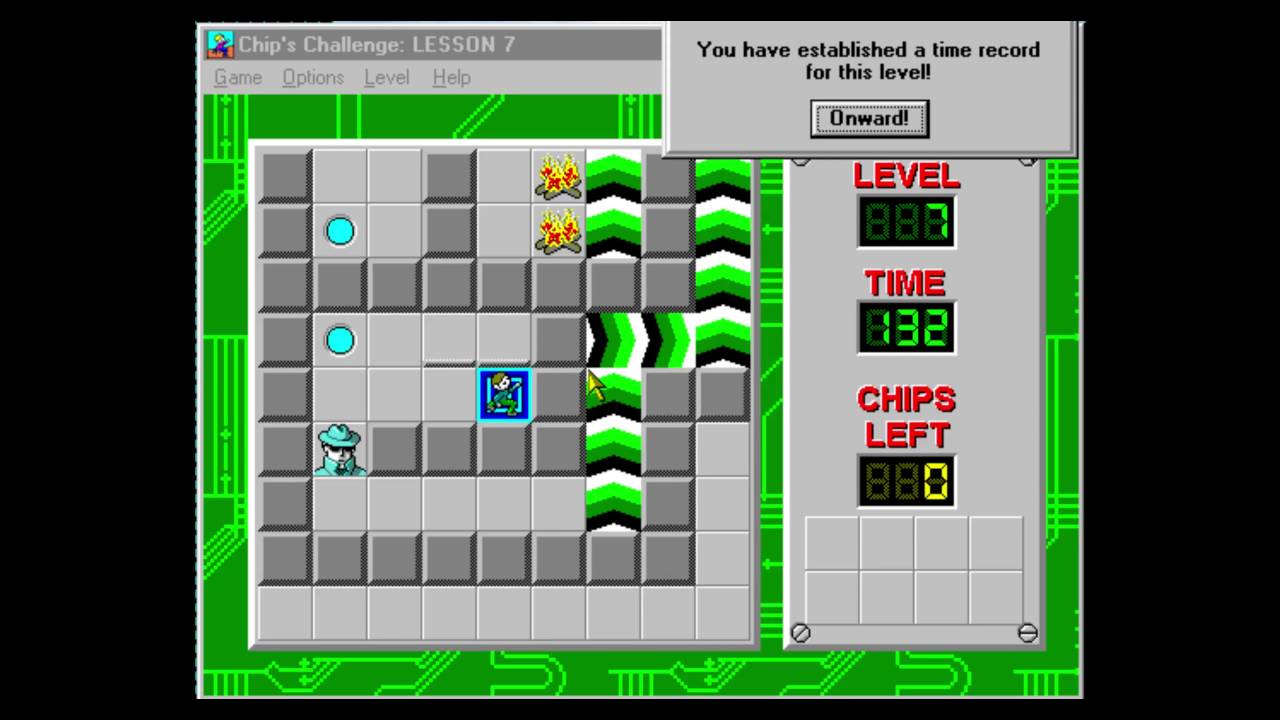
Video: Atari Lynx in action , passing the first level .
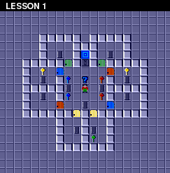
The new game begins with the first level called "LESSON 1". In addition to the chips and the chip connector, keys and doors appear on it. At other levels, obstacles such as traps, bombs, water and creatures arise that (most often) move along predictable routes. A wide range of objects and devices allows you to create many puzzles and time limits. To complete the game you need to go through more than 140 levels.
Although Lynx eventually failed, the Chip's Challenge turned out to be quite popular and was ported to many other platforms, eventually appearing on Microsoft Windows, where it became widespread. A small but loyal fan base formed around the game, and over time a level editor was written that allowed players to create innumerable levels.
And this is where my story begins. I decided that I wanted to create an open source version of the base game engine so that I could play Chip's Challenge on Linux and Windows, and simplify the launch of all levels created by fans.
The existence of a level editor turned out to be a miracle for me, because I could explore the hidden features of the logic of the game, creating my own levels and conducting tests. Unfortunately, there was no level editor for the original game on Lynx, it appeared only in the more well-known port under Windows.
The port under Windows was not created by the original developers, so many changes to the game logic appeared in it (and not all of them were intentional). When I started writing my own engine, I wanted to recreate in it the logic of the original game on Lynx, and the more well-known version under Windows. But the lack of a level editor on Lynx seriously limited my ability to explore the original game in detail. The port under Windows had an advantage: the levels were stored in a separate data file, which simplified its detection and reverse engineering. The game under Lynx was distributed on ROM-cartridges containing sprite images, sound effects and machine code, as well as data levels, which were performed all together. There are no hints about where the data is located in this 128-kilobyte ROM dump, or what it looks like, and without this knowledge I could not create a level editor for the version on Lynx.
Once in the process of leisurely research, I came across a copy of the port of Chip's Challenge under MS-DOS. As in most of the early ports of the game, its logic was closer to the original than in the version for Windows. When I looked at these programs to find out how they are stored, I was surprised to find that these levels were allocated in a separate directory, and each level was stored in its own file. Having such conveniently separated level data, I assumed that it would not be too difficult to perform reverse-engineering of level data files. And this will allow you to write a level editor for the version of the game under MS-DOS. I decided that this is an interesting opportunity.
But then another member of the Chip's Challenge community warned me about an interesting fact. The contents of the level files for MS-DOS turned out to be a single byte ROM Lynx dump. This meant that if I could decode the MS-DOS files, then I would then be able to use this knowledge to read and change the levels inside the ROM Lynx dump. Then you can create a level editor directly for the original game on Lynx.
Suddenly, reverse engineering of level files for MS-DOS became my main priority.
Data files
Here is a link to the tarball directory containing all the data files. I give it in case you want to repeat all the steps described in this article, or try to decode the data files yourself.
Is it legal? Good question. Since these files are only a small part of the MS-DOS program, and they are useless by themselves, and since I post them only for educational purposes, I believe that this falls under fair use requirements. I hope all the interested parties will agree with me. (If, after all, I receive a threatening letter from lawyers, I can change the article to put the data files in an amusing key, and then declare that this is a parody.)
Prerequisites
I will assume that you know hexadecimal calculus, even if you don’t know how to decode hexadecimal values, and that you are a little familiar with the Unix command shell. The shell session shown in this article runs on a standard Linux system, but almost-used commands are common Unix utilities, and are widely distributed on other Unix-like systems.
First look
Here is the listing of the directory containing the data files from the port under MS-DOS:
As you can see, all files end in$ ls levels all_full.pak cake_wal.pak eeny_min.pak iceberg.pak lesson_5.pak mulligan.pak playtime.pak southpol.pak totally_.pak alphabet.pak castle_m.pak elementa.pak ice_cube.pak lesson_6.pak nice_day.pak potproproppropppropp. pak special.pak traffic_.pak amsterda.pak catacomb.pak fireflie.pak icedeath.pak lesson_7.pak nightmar.pak problems.pak spirals.pak trinity.pak apartmen.pak cellbloc.pak firetrap.pak icehouse.pak lesson_8.pak now_you_ .pak refracti.pak spooks.pak trust_me.pak arcticfl.pak chchchip.pak floorgas.pak invincib.pak lobster_.pak nuts_and.pak reverse_.pak steam.pak undergro.pak balls_o_.pak chiller.pak forced_e.pak i.pak lock_blo.pak on_the_r.pak rink.pak stripes.pak up_the_b.pak beware_o.pak chipmine.pak force_fi.pak i_slide.pak loop_aro.pak oorto_ge.pak roadsign.pak suicide.pak vanishin.pak blink.pak mad. pak jailer.pak memory.pak open_que.pak sampler.pak telebloc.pak victim.pak blobdanc.pak colony.pak fortune_.pak jumping_.pak metastab.pak oversea_.pak scavenge.p ak telenet.pak vortex.pak blobnet.pak corridor.pak four_ple.pak kablam.pak mind_blo.pak pain.pak scoundre.pak t_fair.pak wars.pak block_fa.pak cypher.pak four_squ.pak knot.pak mishmeshppakkot.pak mishmeshp .pak seeing_s.pak the_last.pak writers_.pak block_ii.pak deceptio.pak glut.pak ladder.pak miss_dir.pak partial_.pak short_ci.pak the_mars.pak yorkhous.pak block_n_.pak deepfree.pak goldkey.pak mixed_nu.pak pentagra.pak shrinkin.pak the_pris.pak block_ou.pak digdirt.pak go_with_.pak lesson_1.pak mix_up.pak perfect_.pak skelzie.pak three_do.pak block.pak digger.pak grail.pak lesson_2.pak pak pier_sev.pak slide_st.pak time_lap.pak bounce_c.pak doublema.pak hidden_d.pak lesson_3.pak morton.pak ping_pon.pak slo_mo.pak torturec.pak brushfir.pak drawn_an.pak hunt.pak lesson_4.pak mugger_.pak .pak socialis.pak tossed_s.pak
.pak . .pak is the standard resolution for the application data file, and this, unfortunately, does not give us any information about its internal structure. File names are the first eight characters of the level name, with some exceptions. (For example, the word “buster” is omitted from the file names of the “BLOCK BUSTER” and “BLOCK BUSTER II” levels so that they do not match.) $ ls levels | wc
17,148 1974 Now let's examine what these files are.
xxd is a standard utility for dumping hex data (hexdump). Let's see what it looks like inside LESSON 1.$ xxd levels / lesson_1.pak 00000000: 1100 cb00 0200 0004 0202 0504 0407 0505 ................ 00000010: 0807 0709 0001 0a01 010b 0808 0d0a 0a11 ................ 00000020: 0023 1509 0718 0200 2209 0d26 0911 270b. # ...... ".. & .. '. 00000030: 0b28 0705 291e 0127 2705 020d 0122 0704. (..) ..''.... ".. 00000040: 0902 090a 0215 0426 0925 0111 1502 221d ....... &.% .... ". 00000050: 0124 011d 0d01 0709 0020 001b 0400 1a00. $ ....... ...... 00000060: 2015 2609 1f00 3300 2911 1522 2302 110d. & ... 3.) .. "# ... 00000070: 0107 2609 1f18 2911 1509 181a 0223 021b .. & ...) ...... # .. 00000080: 0215 2201 1c01 1c0d 0a07 0409 0201 0201 .. "............. 00000090: 2826 0123 1505 0902 0121 1505 220a 2727 (&. # .....! .. ". '' 000000a0: 0b05 0400 060b 0828 0418 780b 0828 0418 ....... (.. x .. (.. 000000b0: 700b 0828 0418 6400 1710 1e1e 1a19 0103 p .. (.. d ......... 000000c0: 000e 1a17 1710 0e1f 010e 1314 1b29 1f1a .............) .. 000000d0: 0012 101f 011b 0c1e 1f01 1f13 1001 0e13 ................ 000000e0: 141b 001e 1a0e 1610 1f2d 0020 1e10 0116 .........-. .... 000000f0: 1024 291f 1a01 1a1b 1019 000f 1a1a 1d1e. $) ............. 00000100: 2d02
What is a hexdump utility? Hexadecimal dump is a standard way to display exact bytes of a binary file. Most byte values cannot be associated with printable ASCII characters, or they have an incomprehensible appearance (for example, a tab character). In the hexadecimal dump, individual bytes are output as numerical values. Values are displayed in hexadecimal, hence the name. In the example shown above, 16 bytes are displayed on one output line. The leftmost column shows the position of the line in the file, also in hexadecimal, so the number in each line is increased by 16. The bytes are displayed in eight columns, and in each column two bytes are displayed. On the right in hexdump it is shown how the bytes would look when displayed with characters, only all non-printing ASCII values are replaced by dots. This makes it easy to find strings that can be embedded in a binary file.Obviously, the reverse engineering of these files will not be reduced to the usual viewing of the contents and the study of what is visible there. So far, there is nothing telling us which functions are performed by the data.
What do we expect to see?
Let's take a step back and clarify the situation: what specific data do we expect to find in these data files?
The most obvious is a kind of "map" of the level: data indicating the positions of the walls and doors, as well as everything else that makes the level unique.
(Luckily for us, the fans of the game did a good job and collected complete maps for all 148 levels, so we can use them to know what should be on each map.)
In addition to the map, each level should have several other attributes. For example, you may notice that each level has a name, for example “LESSON 1”, “PERFECT MATCH”, “DRAWN AND QUARTERED”, and so on. Different levels also have different time limits, so we can assume that this information is also contained in the data. In addition, each level has its own number of collected chips. (We could assume that this number simply corresponds to the number of chips at the level, but it turns out that at some levels there are more chips than are needed to open the chip connector. At least for these levels the minimum number should be explicitly indicated.)
Another piece of data that we expect to find in the level data is the text of hints. On some levels there is a “hint button” - a large question mark lying on the ground. When Chip gets up on it, the text of the tooltip is shown. The hint button is on about 20 levels.
Finally, each level has a password - a sequence of four letters, which allows the player to continue the game from this level. (This password is necessary because there is no data storage in Lynx. It was impossible to save games on the console, so it was possible to continue the game after turning on the console using passwords.)
So here is our list of relevant data:
- Level map
- Level name
- Password level
- Time limit
- Number of chips
- Help text
Let's roughly estimate the total size of the data. The easiest way to determine the time limit and the number of chips. Both of these parameters can have values ranging from 0 to 999, so they are most likely stored as integer values with a total size of 4 bytes. The password always consists of four letters, so most likely it is stored as four more bytes, that is, only 8 bytes. The length of the names of levels varies from four to nineteen characters. If we assume that we need another byte to complete the string, then it is twenty bytes, that is, the intermediate total is 28 bytes. The longest help text is larger than 80 bytes; if we round this value to 90, then we get 118 bytes in total.
What about the level scheme? Most levels have a size of 32 × 32 tiles. There are no larger levels. Some levels are less, but it will be logical to assume that they are simply embedded in a 32 × 32 map. Assuming that one byte map requires one byte, then the full scheme requires 1024 bytes. That is, in general, we get a rough estimate of 1142 bytes for each level. Of course, this is just a rough initial estimate. It is possible that some of these elements are stored differently, or not at all stored within the level files. Or they may contain other data that we have not noticed or do not know about them. But for now we have laid a good foundation.
Having decided on what we expect to see in the data files, let's go back to exploring what they actually contain.
What is there and what is not
Although at first glance the data file looks completely incomprehensible, you can still notice a couple of moments in it. First, this is what we do not see. For example, we do not see the names of the level or the text of hints. It can be understood that this is not a coincidence by examining other files:
There is nothing visible except arbitrary fragments of ASCII garbage.$ strings levels / * | less : !!; # &> '' :: 4 # . ,,! -54 "; / & 67 !) 60 <171 * (0 * 82> '= / 8> <171 && 9> # 2 ') ( , )9 0hX `@PX ) "" * 24 ** 5 ;)) < B777: .. 22C1 E ,, F -GDED EGFF16G ;; H < IECJ 9K444 = MBBB >> N9 "O" 9P3? Q lines 1-24 / 1544 (more)
Presumably, somewhere in these files there are level names and hints, but they are either not stored in ASCII, or have undergone some kind of transformation (for example, due to compression).
It is also worth noting the following: the file just falls short in size to 256 bytes. This is quite small, given that we initially estimated its size to be more than 1,140 bytes.
The
-S option sorts files in descending order of size.$ ls -lS levels | head total 592 -rw-r - r-- 1 breadbox breadbox 680 Jun 23 2015 mulligan.pak -rw-r - r-- 1 breadbox breadbox 675 Jun 23 2015 shrinkin.pak -rw-r - r-- 1 breadbox breadbox 671 Jun 23 2015 balls_o_.pak -rw-r - r-- 1 breadbox breadbox 648 Jun 23 2015 cake_wal.pak -rw-r - r-- 1 breadbox breadbox 647 Jun 23 2015 citybloc.pak -rw-r - r-- 1 breadbox breadbox 639 Jun 23 2015 four_ple.pak -rw-r - r-- 1 breadbox breadbox 636 Jun 23 2015 trust_me.pak -rw-r - r-- 1 breadbox breadbox 625 Jun 23 2015 block_n_.pak -rw-r - r-- 1 breadbox breadbox 622 Jun 23 2015 mix_up.pak
The largest file takes only 680 bytes, and this is not very much. And what will be the smallest?
The
-r option tells ls to reverse the order.$ ls -lSr levels | head total 592 -rw-r - r-- 1 breadbox breadbox 206 Jun 23 2015 kablam.pak -rw-r - r-- 1 breadbox breadbox 214 Jun 23 2015 fortune_.pak -rw-r - r-- 1 breadbox breadbox 219 Jun 23 2015 digdirt.pak -rw-r - r-- 1 breadbox breadbox 226 Jun 23 2015 lesson_2.pak -rw-r - r-- 1 breadbox breadbox 229 Jun 23 2015 lesson_8.pak -rw-r - r-- 1 breadbox breadbox 237 Jun 23 2015 partial_.pak -rw-r - r-- 1 breadbox breadbox 239 Jun 23 2015 knot.pak -rw-r - r-- 1 breadbox breadbox 247 Jun 23 2015 cellbloc.pak -rw-r - r-- 1 breadbox breadbox 248 Jun 23 2015 torturec.pak
The smallest file takes up only 206 bytes, which is more than three times smaller than the largest. This is a fairly wide interval, taking into account the fact that we expected approximately the same level sizes.
In our initial assessment, we assumed that the map would require one byte per tile, and only 1024 bytes. If we cut this estimate in half, that is, each tile requires only 4 bits (or two tiles per byte), the card will still occupy 512 bytes. 512 is less than 680, but still larger than most levels. And in any case - 4 bits will provide only 16 different values, and in the game there are much more different objects.
That is, it is obvious that maps are not stored in these files in clear text. They use either more complex coding, providing a more efficient description, and / or they are somehow compressed. For example, in the “LESSON 1” level, we can see how missing entries for “empty” tiles will significantly reduce the total size of map data.
We can look at maps of the largest files:
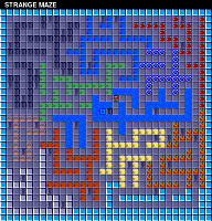
Level 57 card: STRANGE MAZE
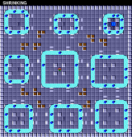
Level 98 map: SHRINKING
and then compare them with maps of the smallest files:
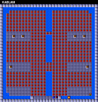
Level 106 map: KABLAM
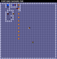
Level 112 card: FORTUNE FAVORS THE
This comparison supports our idea that small data files correspond to simpler levels, or contain more redundancy. For example, if the data is compressed by some run-length encoding, it can easily explain the size intervals of different files.
If the files are actually encrypted, then we will most likely have to decrypt the compression before we begin to decrypt the card data.
We study several files at the same time
Our brief study of the first data file allowed us to make some assumptions, but found nothing concrete. As a next step, we will start exploring the patterns of several data files. For now, we assume that all 148 files use the same ordering scheme for encoding data, so a search for duplicate patterns in these files will help us get to work.
Let's start from the beginning of the tiles. The top of the file is most likely used to store “metadata” that tells us about the contents of the file. Looking only at the first line of the hexadecimal dump, we can perform a simple and quick comparison of the first 16 bytes and search for the patterns in them:
  $ for f in levels / *;  do xxd $ f |  sed -n 1p;  done |  less
 00000000: 2300 dc01 0300 0004 0101 0a03 030b 2323 # ............. ##
 00000000: 2d00 bf01 0300 0015 0101 2203 0329 2222 -......... "..)" "
 00000000: 2b00 a101 0301 0105 0000 0601 0207 0505 + ...............
 00000000: 1d00 d300 0200 0003 0101 0402 0205 0102 ................
 00000000: 2d00 7a01 0300 0006 1414 0701 0109 0303 -.z .............
 00000000: 3100 0802 0200 0003 0101 0502 0206 1313 1 ...............
 00000000: 1a00 b700 0200 0003 0100 0502 0206 0101 ................
 00000000: 1a00 0601 0300 0005 0001 0601 0107 0303 ................
 00000000: 2000 7a01 0200 0003 0202 0401 0105 0028 .z ............ (
 00000000: 3a00 a400 0200 0003 2828 0428 0205 0303: ....... ((. (....
 00000000: 2600 da00 0300 0004 0507 0901 010a 0303 & ...............
 00000000: 2400 f000 0300 0004 0303 0504 0407 0101 $ ...............
 00000000: 2a00 ef01 0300 0005 0101 0614 0007 0303 * ...............
 00000000: 2c00 8c01 0300 0004 0303 0500 0107 0101, ...............
 00000000: 2a00 0001 0300 0004 0303 0501 0107 0404 * ...............
 00000000: 1b00 6d01 0200 0003 0101 0502 0206 0003 ..m .............
 00000000: 1e00 1701 0200 0003 0202 0401 0105 0013 ................
 00000000: 3200 ee01 0f00 0015 0101 270f 0f29 1414 2 ......... '..) ..
 00000000: 2a00 5b01 0300 0005 0303 0601 0107 1414 *. [.............
 00000000: 2c00 8a01 0200 0003 0202 0401 0105 0303, ...............
 00000000: 1d00 9c00 0216 1604 0000 0516 0107 0205 ................
 00000000: 2000 e100 0200 0003 0101 0402 0205 0303 ...............
 00000000: 2000 2601 0300 0004 0303 0502 0207 0101. & .............
 00000000: 1f00 f600 0132 0403 0000 0532 3206 0404 ..... 2 ..... 22 ...
 lines 1-24 / 148 (more)
Looking at this dump, you can see that in each column there are some similar values.
Starting from the first byte, we soon realize that its value lies in a very limited range of values, within
10 to 40 hexadecimal (or approximately 20–60 in decimal). This is a rather specific feature.More interestingly, the second byte of each file is always zero, with no exceptions. Probably, the second byte is not used, or is a placeholder. However, there is another possibility - these first two bytes together denote a 16-bit value stored in little-endian order.
What is little-endian? When saving a numerical value that is more than one byte, you need to select in advance the order in which the bytes will be stored. If you first save a byte representing the smaller part of a number, then this is called direct order ( little-endian ); if you first save the bytes that represent most of the number, then this is the reverse order ( big-endian ). For example, we write decimal values in the reverse order (big-endian): the string "42" means "forty-two", and not "four and twenty". Little-endian is a natural order for many microprocessor families, so it is usually more popular, with the exception of network protocols, which usually require big-endian.
If we continue the analysis, we will soon see that the third byte in the file is not similar to the two previous ones: its value varies in a wide range. However, the fourth byte is always
00 , 01 or 02 , and 01 is most common. This also hints to us that these two bytes make up another 16-bit value, which is approximately in the range of 0–700 decimal values. This hypothesis can also be confirmed by the fact that the value of the third byte is usually low if the value of the fourth is 02 , and is usually large if the fourth byte is 00 .By the way, it is worth noting that this is partly the reason that the standard format of hexadecimal dump displays bytes in pairs - this makes it easier to read a sequence of 16-bit integer numbers. The hex dump format was standardized when 16-bit computers were running. Try replacing
xxd with xxd -g1 to completely disable grouping, and you will notice that the recognition of pairs of bytes in the middle of the line requires a lot of effort. This is a simple example of how the tools used to study unfamiliar data incline us to notice certain types of patterns. It’s good that by default xxd highlights this pattern, because it is very common (even today, when 64-bit computers are used everywhere). But it is useful and to know how to change these parameters if they do not help.Let's continue the visual study, and see if this pattern is preserved from 16-bit integer values. The fifth byte usually has very low values: most often
02 and 03 , and the maximum value seems to be 05 . The sixth byte of a file is very often zero - but sometimes it contains much larger values, for example 32 or 2C . In this pair, our assumption about the values distributed in the interval is not particularly confirmed.We study the original values more closely.
We can test our guess using
od to generate a hex dump. The od utility is similar to xxd , but provides a much larger selection of output formats. We can use it to dump the output as 16-bit decimal integers:The
od option of the od utility indicates the output format. In this case, u stands for unsigned decimal numbers, and 2 stands for two bytes per record. (You can also set this format with the -d option.)$ for f in levels / *; do od -tu2 $ f | sed -n 1p; done | less 0000000 35 476 3 1024 257 778 2819 8995 0000000 45 447 3 5376 257 802 10499 8738 0000000 43 417 259 1281 0 262 1794 1285 0000000 29 211 2 768 257 516 1282 513 0000000 45 378 3 1536 5140 263 2305 771 0000000 49 520 2 768 257 517 1538 4883 0000000 26 183 2 768 1 517 1538 257 0000000 26 262 3 1280 256 262 1793 771 0000000 32 378 2 768 514 260 1281 10240 0000000 58 164 2 768 10280 10244 1282 771 0000000 38 218 3 1024 1797 265 2561 771 0000000 36 240 3 1024 771 1029 1796 257 0000000 42 495 3 1280 257 5126 1792 771 0000000 44 396 3 1024 771 5 1793 257 0000000 42 256 3 1024 771 261 1793 1028 0000000 27 365 2 768 257 517 1538 768 0000000 30 279 2 768 514 260 1281 4864 0000000 50 494 15 5376 257 3879 10511 5140 0000000 42 347 3 1280 771 262 1793 5140 0000000 44 394 2 768 514 260 1281 771 0000000 29 156 5634 1046 0 5637 1793 1282 0000000 32 225 2 768 257 516 1282 771 0000000 32,294 3 1024 771 517 1794 257 0000000 31 246 12801 772 0 12805 1586 1028 lines 1-24 / 148 (more)
This output shows that our first few bytes were correct. We see that the first 16-bit value is in the decimal interval of 20–70, and the second 16-bit value is in the decimal interval of 100–600. However, the following values do not behave so well. Certain patterns appear in them (for example, 1024 is surprisingly often found in the fourth position), but they do not have the repeatability inherent in the first values of the file.
Therefore, let's first assume that the first four bytes of the file are special and consist of two 16-bit values. Since they are at the very beginning of the file, they are likely to be metadata and help determine how to read the rest of the file.
In fact, the second interval of values (100–600) is quite close to the interval of file sizes (208–680) that we noticed earlier. Perhaps this is not a coincidence? Let's hypothesize that the 16-bit value stored in the third and fourth bytes of a file correlates with the overall file size. Now that we have a hypothesis, we can test it. Let's see if large files in this place really have big values, and small ones have small ones.
To display the file size in bytes without any other information, you can use
wc with the option -c . Similarly, you can add to od options that allow you to display only values that interest us. Then we can use command substitution to write these values to shell variables and display them together:The
-An utility option -An disables the leftmost column, which displays the offset in the file, and -N4 tells od stop after the first 4 bytes of the file.$ for f in levels / *; do size = $ (wc -c <$ f); data = $ (od -tuS -An -N4 $ f); echo "$ size: $ data"; done | less 585: 35,476 586: 45 447 550: 43,417 302: 29,211 517: 45 378 671: 49,520 265: 26,183 344: 26,262 478: 32,378 342: 58,164 336: 38,218 352: 36,240 625: 42,495 532: 44,396 386: 42,256 450: 27,365 373: 30 279 648: 50,494 477: 42 347 530: 44,394 247: 29,156 325: 32,225 394: 32,294 343: 31,246
Looking at this output, you can see that the values are approximately correlated. Smaller files usually have smaller values in the second position, and larger files larger ones. However, the correlation is not exact, and it is worth noting that the file size is always significantly larger than the value stored in it.
In addition, the first 16-bit value is also usually larger with large file sizes, but the match is also not entirely complete, and you can easily find examples of medium-sized files with relatively large values in the first position. But maybe if we add up these two values, their sum will be better correlated with the file size?
We can use
readto extract two numbers from the output odinto separate variables, and then use command shell arithmetic to find their sum:Shell command
readcannot be used from the right side of the vertical line, because the commands transmitted to the pipeline are executed in a child command processor (subshell), which, when exiting, takes its environment variables to the bit receiver. Therefore, instead, we need to use the process substitution function bashand send the output odto a temporary file, which can then be redirected to the command read.$ for f in levels / *; do size = $ (wc -c <$ f); read v1 v2 <<(od -tuS -An -N4 $ f); sum = $ (($ v1 + $ v2));
echo "$ size: $ v1 + $ v2 = $ sum"; done | less
585: 35 + 476 = 511
586: 45 + 447 = 492
550: 43 + 417 = 460
302: 29 + 211 = 240
517: 45 + 378 = 423
671: 49 + 520 = 569
265: 26 + 183 = 209
344: 26 + 262 = 288
478: 32 + 378 = 410
342: 58 + 164 = 222
336: 38 + 218 = 256
352: 36 + 240 = 276
625: 42 + 495 = 537
532: 44 + 396 = 440
386: 42 + 256 = 298
450: 27 + 365 = 392
373: 30 + 279 = 309
648: 50 + 494 = 544
477: 42 + 347 = 389
530: 44 + 394 = 438
247: 29 + 156 = 185
325: 32 + 225 = 257
394: 32 + 294 = 326
343: 31 + 246 = 277
lines 1-24 / 148 (more) The sum of the two numbers is also approximately correlated with the file size, but they still do not quite coincide. How different are they? Let's demonstrate their difference:
$ for f in levels / *; do size = $ (wc -c <$ f); read v1 v2 <<(od -tuS -An -N4 $ f); diff = $ (($ size - $ v1 - $ v2));
    echo "$ size = $ v1 + $ v2 + $ diff"; done | less
585 = 35 + 476 + 74
586 = 45 + 447 + 94
550 = 43 + 417 + 90
302 = 29 + 211 + 62
517 = 45 + 378 + 94
671 = 49 + 520 + 102
265 = 26 + 183 + 56
344 = 26 + 262 + 56
478 = 32 + 378 + 68
342 = 58 + 164 + 120
336 = 38 + 218 + 80
352 = 36 + 240 + 76
625 = 42 + 495 + 88
532 = 44 + 396 + 92
386 = 42 + 256 + 88
450 = 27 + 365 + 58
373 = 30 + 279 + 64
648 = 50 + 494 + 104
477 = 42 + 347 + 88
530 = 44 + 394 + 92
247 = 29 + 156 + 62
325 = 32 + 225 + 68
394 = 32 + 294 + 68
343 = 31 + 246 + 66
lines 1-24/148 (more)
The difference, or the value of the “remainder”, is displayed in the rightmost part of the output. This value does not quite fall into a permanent pattern, but it seems to remain approximately in a limited range of 40–120. And again, the larger the files, the more usually their residual values are. But sometimes small files also have large residual values, so this is not as constant as we would like.
However, it is worth noting that the values of the residuals are never negative. Therefore, the idea that these two metadata values point to subsections of a file retains its appeal.
(If you are attentive enough, you have already seen something that gives a hint about a still unnoticed connection. If you have not, then continue to read; the secret will soon be revealed.)
Larger cross-file comparisons
At this stage, it would be nice to be able to cross-compare more than 16 bytes at a time. For this we need a different type of visualization. One of the good approaches is to create an image in which each pixel represents a separate byte of one of the files, and color indicates the value of this byte. The image can show a slice of all 148 files at a time, if each data file will be denoted by a single line of image pixels. Since all files are of different sizes, we will take 200 first bytes of each to build a rectangular image.
The easiest way to build an image in grayscale, in which the value of each byte corresponds to different levels of gray. It is very easy to create a PGM file with our data, because the PGM header consists of only ASCII text:
$ echo P5 200 148 255 >hdr.pgm
PGM? PGM, «portable graymap» (« ») — , : ASCII, . — PBM («portable bitmap», « »), 8 , PPM («portable pixmap», « »), 3 .
P5Is the initial signature indicating the format of the PGM files. The next two numbers, 200and 148, set the width and height of the image, and the last 255, indicates the maximum value per pixel. The PGM header ends with a transition to a new line, followed by pixel data. (It is worth noting that the PGM header is most often broken into three separate lines of text, but the PGM standard only requires that the elements be separated by some whitespace.)We can use the utility
headto extract the first 200 bytes from each file:$ for f in levels / *; do head -c200 $ f; done> out.pgm
Then we can concatenate them with a title and create a displayed image:
xview- this is an old program X for displaying images in a window. You can replace it with your favorite image viewer, for example, with the utility displayfrom ImageMagick, but note that there are surprisingly many image viewing utilities that do not accept the image file redirected to the standard input.$ cat hdr.pgm out.pgm | xview / dev / stdin
If you find it difficult to see the details in a dark image, then you can choose a different color scheme. Use the utility
pgmtoppmfrom ImageMagick to convert pixels to a different range of colors. This version will create a “negative” image:$ cat hdr.pgm out.pgm | pgmtoppm white-black | xview / dev / stdin
And this version makes low values yellow and high values blue:
$ cat hdr.pgm out.pgm | pgmtoppm yellow-blue | xview / dev / stdin
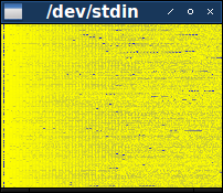
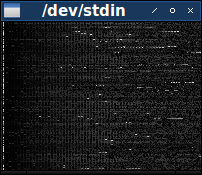
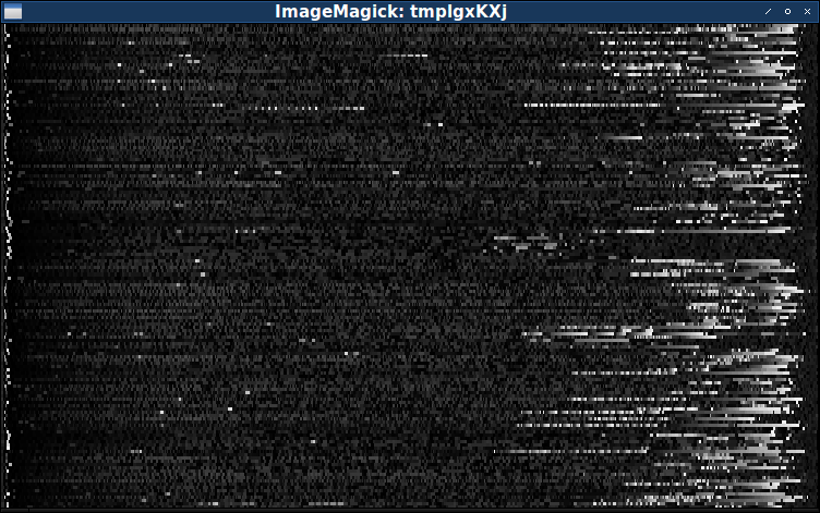
Visibility of colors is a very subjective question, so you can experiment and choose what is best for you. Anyway, the image 200 × 148 is quite small, so it is best to increase the visibility by increasing its size:
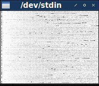
$ cat hdr.pgm out.pgm | xview -zoom 300 / dev / stdin
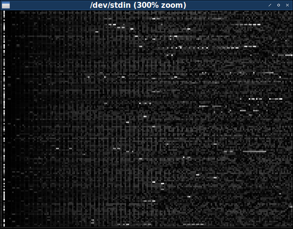
The image is dark, and this means that most bytes contain small values. Contrasts with it a noticeable band of mostly bright pixels closer to the left. This band is located in the third byte of the file, which, as we said above, varies in the full range of values.
And although there are not many high values outside the third byte, when they appear, they often consist of series, creating short bright stripes on the image. Some of these series are periodically interrupted, creating the effect of a dashed line. (Perhaps, with the right selection of colors, it will be possible to notice such sequences in darker colors.)
A careful study of the image can be understood that mainly in the left part is dominated by small vertical stripes. These bands tell us about some repeatability in most files. But not in all the files — from time to time, lines of pixels appear where the stripes are interrupted — but this is more than enough to determine the presence of a real pattern. This pattern disappears on the right side of the image, the dark background of the bands gives way to something more noisy and uncertain. (It seems that the stripes are also missing in the leftmost part of the image, but, again, it is possible that when using a different color scheme, you can see that they start closer to the left edge than it seems here.)
Stripes consist of thin lines of slightly brighter pixels in the background of slightly darker pixels. Consequently, this graphic pattern must correlate with the pattern of data files in which slightly larger values are equally dispersed among slightly smaller byte values. It looks like the stripes are being depleted around the middle of the image. Since it shows the first 200 bytes of files, it should be expected that the byte pattern ends after about 100 bytes.
The fact that these patterns change in different data files should lead us to the question: what files will look like after the first 200 bytes. Well, we can easily replace the utility with the
headutility tailand see what the last 200 bytes look like:$ for f in levels / *; do tail -c200 $ f; done> out.pgm; cat hdr.pgm out.pgm | xview -zoom 300 / dev / stdin
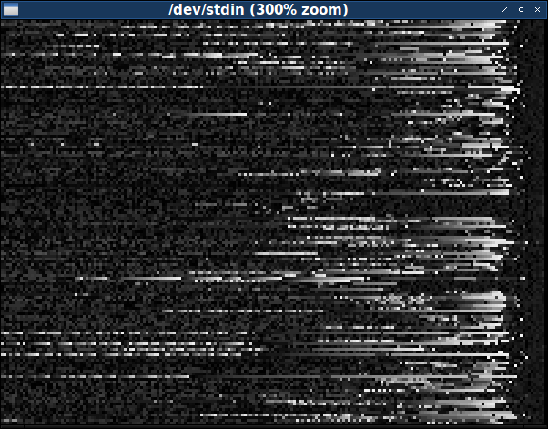
We immediately see that this area of data files is very different. There are much more frequent byte values, especially near the end of the file. (However, as before, they prefer to group together, covering the image with bright horizontal stripes.) It seems that the frequency of high values of bytes increases almost to the very end, where it sharply cuts off and approximately in the last ten to twelve bytes is replaced by low values. And the pattern here is also not universal, but it is too standard to be a coincidence.
Perhaps in the middle of the files there may be other areas that we have not yet considered. The next thing we want to do is examine the entire files in this way. But since all files have different sizes, they cannot be located in a beautiful rectangular array of pixels. We can fill the end of each line with black pixels, but it will be better if we change their size so that all the lines are the same width and the proportional areas of different files more or less coincide.
And we can actually do this with a little more effort. You can use Python and its image library
PIL("Pillow"):Showbytes.py file:
import sys from PIL import Image # Retrieve the full list of data files. filenames = sys.argv[1:] # Create a grayscale image, its height equal to the number of data files. width = 750 height = len(filenames) image = Image.new('L', (width, height)) # Fill in the image, one row at a time. for y in range(height): # Retrieve the contents of one data file. data = open(filenames[y]).read() linewidth = len(data) # Turn the data into a pixel-high image, each byte becoming one pixel. line = Image.new(image.mode, (linewidth, 1)) linepixels = line.load() for x in range(linewidth): linepixels[x,0] = ord(data[x]) # Stretch the line out to fit the final image, and paste it into place. line = line.resize((width, 1)) image.paste(line, (0, y)) # Magnify the final image and display it. image = image.resize((width, 3 * height)) image.show() When we call this script using the full list of data files as arguments, it will create a complete image and display it in a separate window:
$ python showbytes.py levels / *
Unfortunately, although this image is complete, it does not show us anything new. (And in fact, it shows even less, because resizing destroyed the pattern of stripes.) Probably, to study the whole set of data, we will need a better visualization process.
Characterize the data
Taking this into account, let's briefly stop and perform a complete census of data. We need to know if data files give preference to certain byte values. For example, if each value is usually equally repetitive, then this will be strong evidence that the files are actually compressed.
For a complete census of values, just a few lines in Python are enough:
File census.py:
import sys data = sys.stdin.read() for c in range(256): print c, data.count(chr(c)) Storing all the data in one variable, we can calculate the frequency of occurrence of each byte value.
$ cat levels / * | python ./census.py | less
0 2458
1 2525
2 1626
3 1768
4 1042
5 1491
6 1081
7 1445
8,958
9 1541
10 1279
11 1224
 12,845
13,908
14,859
15 1022
16 679
17 1087
18,881
19 1116
20,100
21 1189
22 1029
23,733
lines 1-24 / 256 (more)
We see that the most common byte values are 0 and 1, followed by frequency 2 and 3, after which the number continues to decrease (albeit with less constancy). To better visualize this data, we can transfer the output to
gnuplotand turn this census into a histogram:The
-putility option gnuplottells you not to close the window with the schedule after the work is completed gnuplot.$ cat levels / * | python ./census.py | gnuplot -p -e 'plot "-" with boxes'
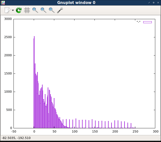
It is very noticeable that the first few byte values are much more common than all the others. The following several values are also quite common, and then the frequencies of values from about 50 begin to decrease along a smooth probability curve. However, there is a subset of high values evenly separated from each other, the frequency of which seems rather stable. Looking at the original output, we can make sure that this subset consists of the values, without dividing by eight.
These differences in the number of values hint that there are several different “classes” of byte values, so it would be logical to see how these classes are distributed. The first group of byte values will be the lowest values: 0, 1, 2 and 3. Then the second group can be values from 4 to 64. And the third group will be values higher than 64, which are completely divided by 8. Everything else, including non-divisible by 8 values greater than 64 will be the fourth and last group.
Given all this, we can change the last written image generation script. Instead of displaying the actual values of each byte in a separate color, let's just show which group each byte belongs to. You can assign a unique color to each of the four groups, and this will help us see if certain values actually appear in certain places.
Showbytes2.py file:
import sys from PIL import Image # Retrieve the full list of data files. filenames = sys.argv[1:] # Create a color image, its height equal to the number of data files. width = 750 height = len(filenames) image = Image.new('RGB', (width, height)) # Fill in the image, one row at a time. for y in range(height): # Retrieve the contents of one data file. data = open(filenames[y]).read() linewidth = len(data) # Turn the data into a pixel-high image, each byte becoming one pixel. line = Image.new(image.mode, (linewidth, 1)) linepixels = line.load() # Determine which group each byte belongs to and assign it a color. for x in range(linewidth): byte = ord(data[x]) if byte < 0x04: linepixels[x,0] = (255, 0, 0) elif byte < 0x40: linepixels[x,0] = (0, 255, 0) elif byte % 8 == 0: linepixels[x,0] = (0, 0, 255) else: linepixels[x,0] = (255, 255, 255) # Paste the line of pixels into the final image, stretching to fit. line = line.resize((width, 1)) image.paste(line, (0, y)) # Magnify the final image and display it. image = image.resize((width, 3 * height)) image.show() We assigned four groups red, green, blue and white colors. (Again, you can try to choose other colors that match your preferences.)
$ python showbytes2.py levels / *
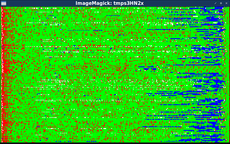
Thanks to this image, we can pre-confirm the correctness of the division of data files into five parts:
- Four-byte header, which we have already found earlier.
- , , (.. ).
- , (. 64).
- , .
- , .
Thanks to these colors, it is clear that in the fourth part, where high byte values prevail, as is seen in the image in grayscale, especially high byte values that divide by 8 predominate.
From the previous image, we know that stretched over an almost completely red area. In fact, in one of the first images we saw that the part with the stripes, going from left to right, on average slowly brightens.
Again, we see that the non-green pixels from the main third part from time to time form dotted patterns of alternating green and red pixels (either blue or white). However, this pattern is not particularly regular, and may be imaginary.
Of course, this division of the file into five parts is very conditional. The fourth part with high byte values, divisible by eight, may be just the end of the third part. Or it may turn out that it is best to divide a large third part into several parts that we have not yet identified. At this stage, the detection of parts more helps us find places for further research. For now, it is enough for us to know that there are parts in which the total composition of byte values changes, and an approximate idea of their size will help us to continue research.
Structure search
What should we look for next? Well, as before, the easiest way is to start from the top of the file. Or rather, near the top. Since we have already quite confidently defined the first part as a four-byte header, let's take a closer look at what comes next - the area that we call the second part, or part of the lanes. These bands are the strongest hint at the existence of a structure, so it is better to look for new evidence for the presence of a pattern here.
(For the time being, we assume that the pattern of bands begins immediately after the first four bytes. Visually, this is not obvious, but it seems likely, and a study of byte values should quickly show us the truth.)
Let's go back to the hex dump, this time focusing on the second part. Remember that we expect to find a repeating pattern of slightly higher values, evenly distributed among slightly lower values.
The option
-s4tells you to xxdskip the first 4 bytes of the file.$ for f in levels / *; do xxd -s4 $ f | sed -n 1p; done | less 00000004: 0200 0003 0202 0401 0105 0303 0700 0108 ................ 00000004: 0201 0104 0000 0504 0407 0202 0902 010a ................ 00000004: 0300 0004 0303 0504 0407 0505 0801 0109 ................ 00000004: 0300 0009 0202 1203 0313 0909 1401 0115 ................ 00000004: 0203 0305 0000 0602 0207 0505 0901 010a ................ 00000004: 0203 0304 0000 0502 0206 0404 0901 010a ................ 00000004: 0300 0005 022a 0602 2907 0303 0902 000a ..... * ..) ....... 00000004: 0203 0305 0000 0605 0507 0101 0802 0209 ................ 00000004: 0300 0007 0303 0901 010a 0707 0b09 090c ................ 00000004: 0300 0004 0101 0903 030e 0404 1609 0920 ............... 00000004: 0200 0003 1313 0402 0205 0013 0701 0109 ................ 00000004: 0500 0006 0505 0701 0109 0606 0e07 070f ................ 00000004: 0100 0003 0101 0a03 030b 0a0a 0e32 3216 .............22. 00000004: 0300 0004 0705 0903 030a 0606 0b08 080c ................ 00000004: 0200 0003 0701 0402 0209 0501 0a08 080b ................ 00000004: 0200 0003 0202 0901 010a 0303 0b05 010d ................ 00000004: 0200 0003 0202 0403 0305 0101 0904 040a ................ 00000004: 0300 0007 0303 0f01 0115 0707 2114 1422 ............!.." 00000004: 0200 0003 0202 0403 0309 0101 0a04 040b ................ 00000004: 0231 3103 0202 0500 0006 0303 0701 0109 .11............. 00000004: 0200 0003 0202 0b32 320c 0303 0e08 0811 .......22....... 00000004: 0201 0103 0000 0902 020a 0303 0b09 090c ................ 00000004: 0200 0003 0202 0a01 010b 0303 0d0b 0b0f ................ 00000004: 0300 0005 0303 0701 0109 0001 0b05 051b ................ lines 27-50/148 (more)
Carefully looking at the sequence of bytes in the string, we can see a pattern in which the first, fourth, seventh and tenth bytes are larger than its nearest neighbors. This pattern is not perfect, there are exceptions in it, but it is definitely stable enough to create the visual repeatability of stripes seen in all images. (And it is enough to confirm our assumption that the strip pattern begins immediately after the four-byte header.) The
constancy of this pattern clearly assumes that this part of the file is an array or a table, and each entry in the array is three bytes long.
You can customize the hex dump format to make it easier to see the output as a series of triplets:
The option
-g3sets the grouping by three bytes instead of two. Option-c18 specifies 18 bytes (a multiple of 3) per line instead of 16.$ for f in levels / *; do xxd -s4 -g3 -c18 $ f | sed -n 1p; done | less 00000004: 050000 060505 070101 090606 0e0707 0f0001 .................. 00000004: 010000 030101 0a0303 0b0a0a 0e3232 161414 ............. 22 ... 00000004: 030000 040705 090303 0a0606 0b0808 0c0101 .................. 00000004: 020000 030701 040202 090501 0a0808 0b0101 .................. 00000004: 020000 030202 090101 0a0303 0b0501 0d0302 .................. 00000004: 020000 030202 040303 050101 090404 0a0302 .................. 00000004: 030000 070303 0f0101 150707 211414 221313 ............! .. ".. 00000004: 020000 030202 040303 090101 0a0404 0b0001 .................. 00000004: 023131 030202 050000 060303 070101 090505 .11 ............... 00000004: 020000 030202 0b3232 0c0303 0e0808 110b0b ....... 22 ......... 00000004: 020101 030000 090202 0a0303 0b0909 0c0a0a .................. 00000004: 020000 030202 0a0101 0b0303 0d0b0b 0f2323 ................## 00000004: 030000 050303 070101 090001 0b0505 1b0707 .................. 00000004: 022323 030000 040202 050303 030101 070505 .##............... 00000004: 031414 050000 060303 070505 080101 090707 .................. 00000004: 030000 050202 060303 070505 080101 090606 .................. 00000004: 030202 040000 050303 070404 080005 090101 .................. 00000004: 030202 040000 050303 090404 1d0101 1f0909 .................. 00000004: 020000 050303 060101 070202 0f0300 110505 .................. 00000004: 050000 070101 0c0505 0d0007 110c0c 120707 .................. 00000004: 030202 050000 060303 070505 080101 090606 .................. 00000004: 020000 030101 050202 060505 070100 080303 .................. 00000004: 020000 030202 050303 090101 0a0505 0b0302 .................. 00000004: 022c2c 030000 040202 020303 050101 060202 .,,............... lines 38-61/148 (more)
Some other features of this pattern begin to appear in the dump formatted in this way. As before, the first byte of each triple is usually more than the surrounding bytes. You may also notice that the second and third bytes of each triplet are often duplicated. Passing down the first column, we see that most of the values of the second and third bytes are equal
0000. But nonzero values are also often found in pairs, for example, 0101or 2323. This pattern is also not ideal, but it has too much in common for it to be a coincidence. And looking at the ASCII column on the right, we will see that when we have byte values that correspond to the printed ASCII character, they are often found in pairs.Another worth mentioning pattern that is not immediately noticeable: the first byte of each triplet increases from left to right. Although this pattern is less noticeable, its stability is high; we need to look at many lines before we find the first discrepancy. And bytes are usually incremented by small values, but they do not represent any regular pattern.
When studying the original image, we noticed that the part with stripes ends in each file not in the same place. There is a transition from the pattern-creating pattern on the left to randomly looking noise on the right, but this transition occurs for each row of pixels at different points. This implies that there must be a certain marker so that the program reading the data file can understand where the array ends and another data set begins.
Let's go back to the first level dump only, to examine the entire file:
 $ xxd -s4 -g3 -c18 levels / lesson_1.pak
00000004: 020000 040202 050404 070505 080707 090001 ..................
00000016: 0a0101 0b0808 0d0a0a 110023 150907 180200 ........... # ......
00000028: 22090d 260911 270b0b 280705 291e01 272705 ".. & .. '.. (..) ..' '.
0000003a: 020d01 220704 090209 0a0215 042609 250111 ... "......... &.% ..
0000004c: 150222 1d0124 011d0d 010709 002000 1b0400 .. ".. $ ....... ....
0000005e: 1a0020 152609 1f0033 002911 152223 02110d ... & ... 3.) .. "# ...
00000070: 010726 091f18 291115 09181a 022302 1b0215 .. & ...) ...... # ....
00000082: 22011c 011c0d 0a0704 090201 020128 260123 "............. (&.
00000094: 150509 020121 150522 0a2727 0b0504 00060b .....! .. ".''......
000000a6: 082804 18780b 082804 18700b 082804 186400 .(..x..(..p..(..d.
000000b8: 17101e 1e1a19 010300 0e1a17 17100e 1f010e ..................
000000ca: 13141b 291f1a 001210 1f011b 0c1e1f 011f13 ...)..............
000000dc: 10010e 13141b 001e1a 0e1610 1f2d00 201e10 .............-.  ..
000000ee: 011610 24291f 1a011a 1b1019 000f1a 1a1d1e ...$).............
00000100: 2d02
Studying the sequences of triplets, we can first assume that the part with the bands in these data ends after 17 triplets, by the offset
00000036. This is not accurate, but the first byte of each triplet constantly increases its value, and then decreases on the eighteenth triplet. Another proof: in the eighteenth triplet, the second byte has the same meaning as the first. We have not noticed this yet, but if we go back and see, we will see that the first byte is never equal to the second or third byte.If our theory about markers is true, then there are two possibilities. Firstly, it is possible that there is some special byte value after the part with stripes (immediately after the seventeenth triplet). Secondly, there is probably a value stored somewhere equal to the size of the part with the stripes. This size can be equal to 17 (that is, indicates the number of triplets), or 51 (indicates the total number of bytes in the part), or 55 (51 plus 4, that is, the offset of the file in which this part ends).
For the first option, a double byte value can be a marker for the end of a part (given that such a sequence never occurs in the second part). However, a careful study of several other data files contradicts this idea, because such a pattern does not appear anywhere else.
For the second option, it will be obvious to look for the size indicator in the first part. Behold - the first 16-bit value in the four-byte file header is 17:
 $ od -An -tuS -N4 levels / lesson_1.pak
    17 203
If our theory is correct, then this value does not determine the size of the part with strips, but the number of three-byte records. To test this idea, let's go back to the calculations, where we compared the sum of two 16-bit integer values with the file size. This time we multiply the first number by three to get the actual size in bytes:
$ for f in levels / *; do size = $ (wc -c <$ f); read v1 v2 <<(od -tuS -An -N4 $ f); diff = $ (($ size - 3 * $ v1 - $ v2));
    echo "$ size = 3 * $ v1 + $ v2 + $ diff"; done | less
585 = 3 * 35 + 476 + 4
586 = 3 * 45 + 447 + 4
550 = 3 * 43 + 417 + 4
302 = 3 * 29 + 211 + 4
517 = 3 * 45 + 378 + 4
671 = 3 * 49 + 520 + 4
265 = 3 * 26 + 183 + 4
344 = 3 * 26 + 262 + 4
478 = 3 * 32 + 378 + 4
342 = 3 * 58 + 164 + 4
336 = 3 * 38 + 218 + 4
352 = 3 * 36 + 240 + 4
625 = 3 * 42 + 495 + 4
532 = 3 * 44 + 396 + 4
386 = 3 * 42 + 256 + 4
450 = 3 * 27 + 365 + 4
373 = 3 * 30 + 279 + 4
648 = 3 * 50 + 494 + 4
477 = 3 * 42 + 347 + 4
530 = 3 * 44 + 394 + 4
247 = 3 * 29 + 156 + 4
325 = 3 * 32 + 225 + 4
394 = 3 * 32 + 294 + 4
343 = 3 * 31 + 246 + 4
lines 1-24/148 (more) AhaAfter this change, the total amount from the header is always exactly four less than the size of the entire data file. And since four is also the number of bytes in the header, this is obviously not a coincidence. The first number gives us the number of three byte records in the table, and the second number gives us the number of bytes that make up the rest of the data file.
We found a constant formula, which means we now fully understand what the numbers in the first part mean.
(By the way, here is the very secret pattern that attentive readers might have noticed. If you carefully study the equations, it becomes clear that when files have the same first number, they get the same difference of the remainder. This happens because the difference is always twice as large as The first number. This is an unobvious pattern, but a painstaking or successful observer might notice it.)
So, we can say that the file has three main parts:
- four byte header;
- three-byte table; and
- the remainder of the file, which presumably contains most of the data.
(Consequently, the other parts that we have roughly identified earlier should be subsections of the third part.)
We interpret metadata
Given this scheme, it would be logical to assume that the entries in the second part table are some kind of metadata that is needed to interpret the third part data.
But what kind of metadata does this table contain?
Above, we noticed that there are a couple of signs that the data file can be compressed. (Now it seems more plausible, because we know that the third part of each file, presumably containing data for each level, is only 100–600 bytes in size.) If this is the case, then it is quite possible that the table that introduces basic data contains compression metadata - a kind of dictionary used during unpacking. For example, before the data encoded by the Huffman algorithm, there is usually a dictionary associating the original byte values with bit sequences. Although we do not expect these files to be encoded with a Huffman algorithm (since the data shows clear patterns at the byte level, that is, hardly a bitstream), it would be reasonable to try to interpret this table as an unpacking dictionary.
(Of course, not every type of compression uses a stored dictionary. For example, the deflate algorithm used in
gzipand zliballows you to recreate a dictionary directly from the data stream. But such cases are the exception rather than the rule.)Typically, a dictionary entry consists of two parts: the key and values. Of course, sometimes the key is implied, for example, when it is ordered not into a lookup table, but into an array. However, we have already noticed that three-byte records seem to consist of two parts - in particular, the first byte of each record follows a pattern that is clearly different from the pattern of the second and third bytes. With this in mind, a reasonable first hypothesis would be to consider the first byte as the key, and the remaining two bytes, the value.
If this is the case, then one of the simplest ways to interpret the part with stripes is that the first byte is the byte value that needs to be replaced in the compressed data, and the second and third byte is the value that needs to be replaced with it. The result created by this scheme will definitely be more, although it is not clear how much. Anyway, this is quite a logical hypothesis, and it is easy enough to test it. We can write a short program in Python that implements this unpacking scheme:
decompress.py file:
import struct import sys # Read the compressed data file. data = sys.stdin.read() # Extract the two integers of the four-byte header. tablesize, datasize = struct.unpack('HH', data[0:4]) data = data[4:] # Separate the dictionary table and the compressed data. tablesize *= 3 table = data[0:tablesize] data = data[tablesize:datasize] # Apply the dictionary entries to the data section. for n in range(0, len(table), 3): key = table[n] val = table[n+1:n+3] data = data.replace(key, val) # Output the expanded result. sys.stdout.write(data) Now we can test this script using the data file example:
$ python ./decompress.py <levels/lesson_1.pak | xxd
00000000: 0b0b 0b0b 0404 0000 0a0a 0109 0d05 0502 ................
00000010: 0200 0100 0000 0101 0100 0009 0702 0209 ................
00000020: 1100 0125 0100 2309 0700 0009 0d1d 0124 ...%..#........$
00000030: 011d 0a0a 0105 0500 0100 2000 1b02 0200 .......... .....
00000040: 1a00 2009 0709 1100 011f 0033 001e 0100 .. ........3....
00000050: 2309 0709 0d23 0000 0023 0a0a 0105 0509 #....#...#......
00000060: 1100 011f 0200 1e01 0023 0907 0001 0200 .........#......
00000070: 1a00 0023 0000 1b00 0009 0709 0d01 1c01 ...#............
00000080: 1c0a 0a01 0105 0502 0200 0100 0001 0000 ................
00000090: 0107 0509 1101 2309 0704 0400 0100 0001 ......#.........
000000a0: 2109 0704 0409 0d01 010b 0b0b 0b08 0804 !...............
000000b0: 0402 0200 0608 0807 0707 0502 0202 0078 ...............x
000000c0: 0808 0707 0705 0202 0200 7008 0807 0707 ..........p.....
000000d0: 0502 0202 0064 0017 101e 1e1a 1901 0300 .....d..........
000000e0: 0e1a 1717 100e 1f01 0e13 141b 1e01 1f1a ................
000000f0: 0012 101f 011b 0c1e 1f01 1f13 1001 0e13 ................
00000100: 141b 001e 1a0e 1610 1f2d 0020 1e10 0116 .........-. ....
00000110: 1024 1e01 1f1a 011a 1b10 1900 0f1a 1a1d .$..............
00000120: 1e2d 0000
However, the results are unremarkable. Of course, the resulting data stream has become more extensive than the original, but not much. Definitely not enough to contain all the data that we expect to find. Obviously, this unpacking scheme is a bit simpler than necessary.
If we carefully examine the output, we will soon see that it begins with a set of repeated bytes.
0b, 04, 00, 0a- they all occur in pairs. Looking at the compressed original, we will see that all these pairs arose because of the replacement by the dictionary. But in the process, we immediately note that all these duplicate values also correspond to entries in the dictionary. That is, if we again apply the dictionary, then the data will expand again. Perhaps we are not unpacking enough?Our first guess can be to perform the second pass, use each dictionary entry a second time to expand the data even more. The second guess can be performing multiple passes with a dictionary, repeating the process, until all bytes that look like dictionary keys are replaced. However, if we take a closer look at the structure of the dictionary, we are aware that we simply use dictionary entries from right to left , rather than from left to right, when all our meanings are deployed in one pass.
Taking this hypothesis, we can see the structure of a more plausible compression algorithm. The program takes the source data and scans it, looking for the most common double-byte sequence. It then replaces the two-byte sequence with a single byte value that is not found in the data. Then it repeats the process, continuing it until there is more than twice the repetition of two-byte sequences in the data. In fact, such a compression algorithm has a name: it is known as “re-pair” compression, which is short for “recursive pairs”.
(And this may explain some patterns that we see in the dictionary. In the process of compression, the dictionary is built from left to right, so when unpacking it should be used from right to left. Since dictionary entries often refer to previous entries, it is logical that the second and third bytes will often be smaller in value than the first.)
Although re-pair compression does not produce particularly impressive results, it has an advantage: the unpacker can be implemented with a minimum of code. I myself used re-pair in some situations when I needed to minimize the total size of the compressed data and the decompression code.
So, we can make a change to one line of the Python program to apply the dictionary from right to left:
decompress2.py file:
import struct import sys # Read the compressed data file. data = sys.stdin.read() # Extract the two integers of the four-byte header. tablesize, datasize = struct.unpack('HH', data[0:4]) data = data[4:] # Separate the dictionary table and the compressed data. tablesize *= 3 table = data[0:tablesize] data = data[tablesize:datasize] # Apply the dictionary entries to the data section in reverse order. for n in range(len(table) - 3, -3, -3): key = table[n] val = table[n+1:n+3] data = data.replace(key, val) # Output the expanded result. sys.stdout.write(data) If we try this version, the output will be much more:
 $ python ./decompress2.py <levels/lesson_1.pak | xxd | less
00000000: 0000 0000 0000 0000 0000 0000 0000 0000 ................
00000010: 0000 0000 0000 0000 0000 0000 0000 0000 ................
00000020: 0000 0000 0000 0000 0000 0000 0000 0000 ................
00000030: 0000 0000 0000 0000 0000 0000 0000 0000 ................
00000040: 0000 0000 0000 0000 0000 0000 0000 0000 ................
00000050: 0000 0000 0000 0000 0000 0000 0000 0000 ................
00000060: 0000 0000 0000 0000 0000 0000 0000 0000 ................
00000070: 0000 0000 0000 0000 0000 0000 0000 0000 ................
00000080: 0000 0000 0000 0000 0000 0000 0000 0000 ................
00000090: 0000 0000 0000 0000 0000 0000 0000 0000 ................
000000a0: 0000 0000 0000 0000 0000 0000 0000 0000 ................
000000b0: 0000 0000 0000 0000 0000 0000 0000 0000 ................
000000c0: 0000 0000 0000 0000 0000 0000 0000 0000 ................
000000d0: 0000 0000 0000 0000 0000 0000 0000 0000 ................
000000e0: 0000 0000 0000 0000 0000 0000 0000 0000 ................
000000f0: 0000 0000 0000 0000 0000 0000 0000 0000 ................
00000100: 0000 0000 0000 0000 0000 0101 0101 0100 ................
00000110: 0101 0101 0100 0000 0000 0000 0000 0000 ................
00000120: 0000 0000 0000 0000 0000 0100 0000 0101 ................
00000130: 0100 0000 0100 0000 0000 0000 0000 0000 ................
00000140: 0000 0000 0000 0000 0000 0100 2300 0125 ............#..%
00000150: 0100 2300 0100 0000 0000 0000 0000 0000 ..#.............
00000160: 0000 0000 0000 0000 0101 0101 011d 0124 ...............$
00000170: 011d 0101 0101 0100 0000 0000 0000 0000 ................
lines 1-24 / 93 (more)
We see in this output a lot of zero bytes, but this may well correspond to an almost empty map. It looks like nonzero bytes are grouped next to each other. Since we hope to find a 32 × 32 map, let's reformat the output to 32 bytes per line:
$ python ./decompress2.py <levels / lesson_1.pak | xxd -c32 | less
00000000: 0000 0000 0000 0000 0000 0000 0000 0000 0000 0000 0000 0000 0000 0000 0000 0000 000000 ................................
00000020: 0000 0000 0000 0000 0000 0000 0000 0000 0000 0000 0000 0000 0000 0000 0000 0000 000000 ................................
00000040: 0000 0000 0000 0000 0000 0000 0000 0000 0000 0000 0000 0000 0000 0000 0000 0000 000000 ................................
00000060: 0000 0000 0000 0000 0000 0000 0000 0000 0000 0000 0000 0000 0000 0000 0000 0000 ................................
00000080: 0000 0000 0000 0000 0000 0000 0000 0000 0000 0000 0000 0000 0000 0000 0000 0000 ................................
000000a0: 0000 0000 0000 0000 0000 0000 0000 0000 0000 0000 0000 0000 0000 0000 0000 0000 ................................
000000c0: 0000 0000 0000 0000 0000 0000 0000 0000 0000 0000 0000 0000 0000 0000 0000 0000 ................................
000000e0: 0000 0000 0000 0000 0000 0000 0000 0000 0000 0000 0000 0000 0000 0000 0000 0000 ................................
00000100: 0000 0000 0000 0000 0000 0101 0101 0100 0101 0101 0100 0000 0000 0000 0000 0000 ................................
00000120: 0000 0000 0000 0000 0000 0100 0000 0101 0100 0000 0100 0000 0000 0000 0000 0000 ................................
00000140: 0000 0000 0000 0000 0000 0100 2300 0125 0100 2300 0100 0000 0000 0000 0000 0000 ............#..%..#.............
00000160: 0000 0000 0000 0000 0101 0101 011d 0124 011d 0101 0101 0100 0000 0000 0000 0000 ...............$................
00000180: 0000 0000 0000 0000 0100 2000 1b00 0000 0000 1a00 2000 0100 0000 0000 0000 0000 .......... ......... ...........
000001a0: 0000 0000 0000 0000 0100 2300 011f 0033 001e 0100 2300 0100 0000 0000 0000 0000 ..........#....3....#...........
000001c0: 0000 0000 0000 0000 0101 0101 0123 0000 0023 0101 0101 0100 0000 0000 0000 0000 .............#...#..............
000001e0: 0000 0000 0000 0000 0100 2300 011f 0000 001e 0100 2300 0100 0000 0000 0000 0000 ..........#.........#...........
00000200: 0000 0000 0000 0000 0100 0000 1a00 0023 0000 1b00 0000 0100 0000 0000 0000 0000 ...............#................
00000220: 0000 0000 0000 0000 0101 0101 0101 1c01 1c01 0101 0101 0100 0000 0000 0000 0000 ................................
00000240: 0000 0000 0000 0000 0000 0000 0100 0001 0000 0100 0000 0000 0000 0000 0000 0000 ................................
00000260: 0000 0000 0000 0000 0000 0000 0100 2301 2300 0100 0000 0000 0000 0000 0000 0000 ..............#.#...............
00000280: 0000 0000 0000 0000 0000 0000 0100 0001 2100 0100 0000 0000 0000 0000 0000 0000 ................!...............
000002a0: 0000 0000 0000 0000 0000 0000 0101 0101 0101 0100 0000 0000 0000 0000 0000 0000 ................................
000002c0: 0000 0000 0000 0000 0000 0000 0000 0000 0000 0000 0000 0000 0000 0000 0000 0000 ................................
000002e0: 0000 0000 0000 0000 0000 0000 0000 0000 0000 0000 0000 0000 0000 0000 0000 0000 ................................
lines 1-24/47 (more)
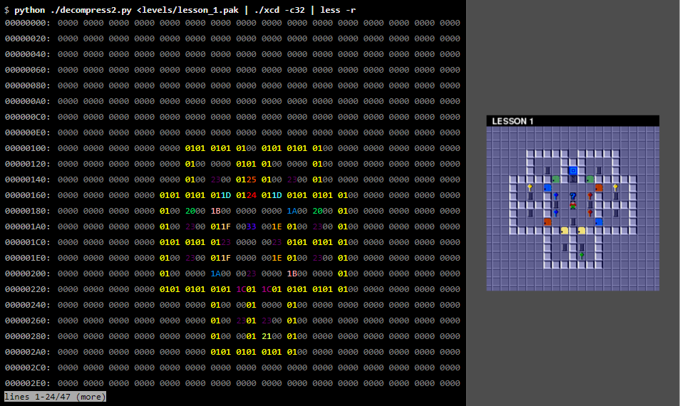
Carefully looking at the patterns of nonzero values, we will see that the map is clearly visible in the output. In fact, we can make this pattern more noticeable with the help of the “colored” dump tool, which assigns its own color to each byte value, making it easier to find patterns of duplicate values:
xcdis a non-standard tool, but you can download it from here . Note the option of the -rutility less, which orders to clear control sequences.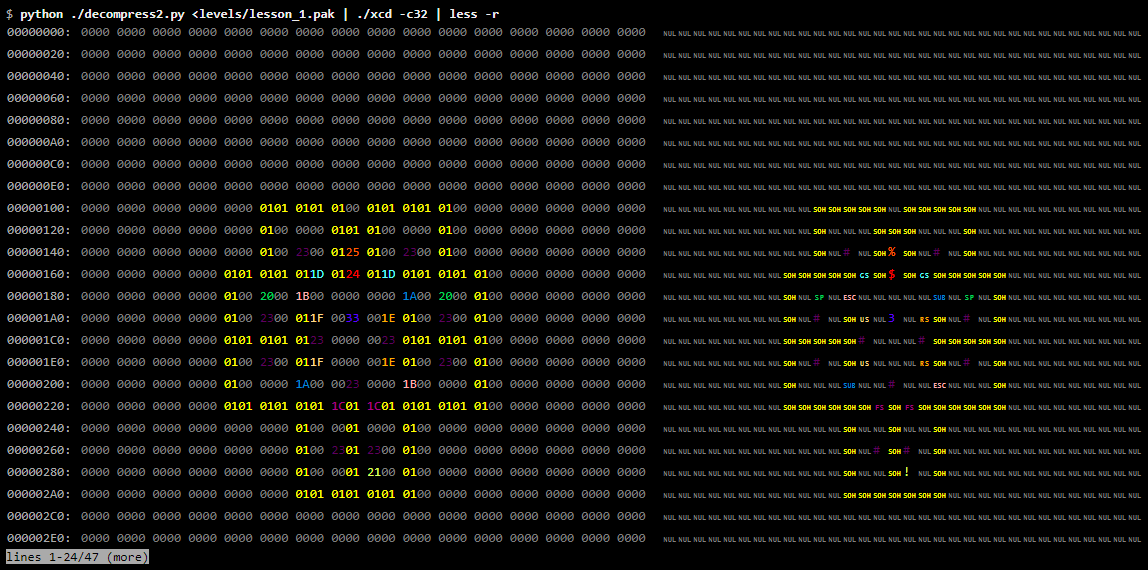
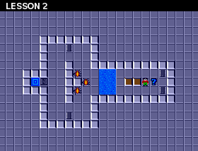
Compare this with the first-level map drawn by fans:
Without a doubt, we see the data card level. You can be quite sure that we correctly identified the decompression algorithm.
Interpreting data
By comparing the byte values with the map image, we can determine what
00encodes an empty tile, 01encodes a wall, and 23denotes a chip. 1Adenotes a red door, 1Ba blue door, and so on. We can assign exact values to chips, keys, doors, and all other tiles that make up the entire level map.Now we can go to the next level and find the byte values for the objects appearing there. And continue with the following levels until we get a complete list of byte values and game objects that they encode.
As we originally assumed, the card ends exactly after 1024 bytes (by offset
000003FF).This time, to remove the first 32 rows of the dump, we use
sed. Since we display 32 bytes per line, so we skip the first 1024 bytes.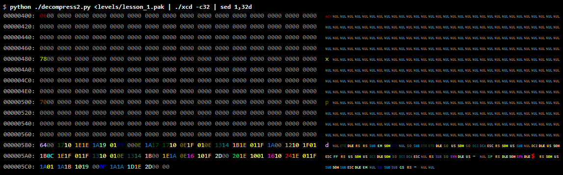
Immediately after the card data, there is a sequence of 384 bytes (the values of which are in the interval
00000400- 0000057F), almost all of which are zero, but nonzero values are found between them. After that there is a completely different byte pattern, so it would be logical to assume that this 384-byte sequence is a separate part.If we look at several more levels, we will quickly notice the pattern. The 384-byte part actually consists of three subsections, each 128 bytes long. Each subsection begins with several non-zero bytes, followed by zeros that fill the remainder of the subsection.
Some levels here contain a lot of data; for others (for example, the first level), only the very minimum. Comparing the levels with their maps, we will soon notice that the amount of data in this part of the file is directly related to the number of “mobs” in the level. In this case, the number of "mobs" includes all creatures at the level, blocks of the earth (which do not move independently, but they can be pushed) and the main character Chip (player) himself. That is, mobs are not indicated on the card itself, but are encoded in these three buffers.
After we learned that these three subsections contain data on the level of mobs, it will not be very difficult to figure out what is contained in each of the subsections.
The first 128-byte subkey is a list of byte values that determine the type of mob. For example, second level buffers look like this:
 $ python ./decompress2.py <levels/lesson_2.pak | xxd | less
00000400: 0608 1c1c 0808 0000 0000 0000 0000 0000 ................
00000410: 0000 0000 0000 0000 0000 0000 0000 0000 ................
00000420: 0000 0000 0000 0000 0000 0000 0000 0000 ................
00000430: 0000 0000 0000 0000 0000 0000 0000 0000 ................
00000440: 0000 0000 0000 0000 0000 0000 0000 0000 ................
00000450: 0000 0000 0000 0000 0000 0000 0000 0000 ................
00000460: 0000 0000 0000 0000 0000 0000 0000 0000 ................
00000470: 0000 0000 0000 0000 0000 0000 0000 0000 ................
00000480: a870 98a0 6868 0000 0000 0000 0000 0000 .p..hh..........
00000490: 0000 0000 0000 0000 0000 0000 0000 0000 ................
000004a0: 0000 0000 0000 0000 0000 0000 0000 0000 ................
000004b0: 0000 0000 0000 0000 0000 0000 0000 0000 ................
000004c0: 0000 0000 0000 0000 0000 0000 0000 0000 ................
000004d0: 0000 0000 0000 0000 0000 0000 0000 0000 ................
000004e0: 0000 0000 0000 0000 0000 0000 0000 0000 ................
000004f0: 0000 0000 0000 0000 0000 0000 0000 0000 ................
00000500: 6060 6060 5868 0000 0000 0000 0000 0000 ````Xh..........
00000510: 0000 0000 0000 0000 0000 0000 0000 0000 ................
00000520: 0000 0000 0000 0000 0000 0000 0000 0000 ................
00000530: 0000 0000 0000 0000 0000 0000 0000 0000 ................
00000540: 0000 0000 0000 0000 0000 0000 0000 0000 ................
00000550: 0000 0000 0000 0000 0000 0000 0000 0000 ................
00000560: 0000 0000 0000 0000 0000 0000 0000 0000 ................
00000570: 0000 0000 0000 0000 0000 0000 0000 0000 ................
lines 64-87 / 93 (more)
Compare this to the level map:
At this level there are six mobs: three beetles, two blocks and a chip. The first 128-byte subkey contains one byte
06, three bytes, 08and two bytes 1C. It will be reasonable to conclude that 06Chip means 08- a beetle, and 1C- a block.(Continuing to compare data files from the levels of the cards and fill in our dictionary mobs, we quickly find a flaw in this theory: The chip may be referred to four different values, namely
04, 05, 06or07. This set of symbols actually contains all mobs. A careful study of different values, we eventually realize that byte value, indicating the type, is added the value 0, 1, 2 or 3, denoting the initial direction of the mob: north, east, south or west. That is, for example, a byte value 06denotes a Chip looking south.)The meaning of the two other subsections is less obvious. But after examining the duplicate values in these subsections and comparing the maps for these mobs, we understand that the bytes in the second subsection store the X coordinate of each mob, and the bytes in the third subsection store the Y coordinate of each mob. Understanding this decision is hampered by the fact that the coordinates stored in these subsections are actually shifted 3 bits to the left, i.e. multiplied by 8. This small fact explains the “blue” group that we found when censoring values. (The reasons that made this shift are not clear, but is likely to lower three bits are used to represent the animation when the mobs move.)
Having dealt with this part, we can now see how many data files left behind her only a few bytes of data:
Note, what
xxdaccepts a -shex value for the option .$ for f in levels / *; do python ./decompress2.py <$ f | xxd -s 0x580 | sed -n 1p; done | less 00000580: 9001 0c17 1701 1120 1717 00 ....... ... 00000580: 0000 0c17 1b13 0c0d 101f 011e 1a20 1b00 ............. .. 00000580: f401 0c18 1e1f 101d 0f0c 1800 ............ 00000580: 2c01 0c1b 0c1d 1f18 1019 1f00, ........... 00000580: 9001 0c1d 0e1f 140e 1117 1a22 00 ........... ". 00000580: 2c01 0d0c 1717 1e01 1a01 1114 1d10 00, .............. 00000580: 2c01 0d10 220c 1d10 011a 1101 0d20 1200, ... "........ .. 00000580: 5802 0d17 1419 1600 X ....... 00000580: 0000 0d17 1a0d 0f0c 190e 1000 ............ 00000580: f401 0d17 1a0d 1910 1f00 .......... 00000580: f401 0d17 1a0e 1601 110c 0e1f 1a1d 2400 .............. $. 00000580: ee02 0d17 1a0e 1601 0d20 1e1f 101d 0114 ......... ...... 00000580: 5802 0d17 1a0e 1601 1901 1d1a 1717 00 X.............. 00000580: 5e01 0d17 1a0e 1601 1a20 1f00 ^........ .. 00000580: c201 0d17 1a0e 1601 0d20 1e1f 101d 00 ......... ..... 00000580: 2c01 0d1a 2019 0e10 010e 141f 2400 ,... .......$. 00000580: 5000 0d1d 201e 1311 141d 1000 P... ....... 00000580: e703 0e0c 1610 0122 0c17 1600 .......".... 00000580: 5802 0e0c 1e1f 1710 0118 1a0c 1f00 X............. 00000580: 8f01 0e0c 1f0c 0e1a 180d 1e00 ............ 00000580: 0000 0e10 1717 0d17 1a0e 1610 0f00 1b1d ................ 00000580: 2c01 0e13 0e13 0e13 141b 1e00 ,........... 00000580: 8f01 0e13 1417 1710 1d00 .......... 00000580: bc02 0e13 141b 1814 1910 00 ........... lines 1-24/148 (more)
Studying the first pair of bytes in the remainder quickly hints to us that they contain another 16-bit integer value. If we read them like this, then most of the values are in decimal notation with round numbers:
The command
oduses the command to go to the original offset -jinstead -s. It is also worth noting the command printf: in addition to providing formatting, it is a convenient way to display text without a new line hanging at the end of the character.$ for f in levels / *; do printf "% -20s" $ f; python ./decompress2.py <$ f | od -An -j 0x580 -tuS -N2; done | less levels / all_full.pak 400 levels / alphabet.pak 0 levels / amsterda.pak 500 levels / apartmen.pak 300 levels / arcticfl.pak 400 levels / balls_o_.pak 300 levels / beware_o.pak 300 levels / blink.pak 600 levels / blobdanc.pak 0 levels / blobnet.pak 500 levels / block_fa.pak 500 levels / block_ii.pak 750 levels / block_n_.pak 600 levels / block_ou.pak 350 levels / block.pak 450 levels / bounce_c.pak 300 levels / brushfir.pak 80 levels / cake_wal.pak 999 levels / castle_m.pak 600 levels / catacomb.pak 399 levels / cellbloc.pak 0 levels / chchchip.pak 300 levels / chiller.pak 399 levels / chipmine.pak 700 lines 1-24 / 148 (more)
If we again refer to the list originally created from the data that was expected to be found in the files, then we realize that this number is the time for passing the level (if the value is zero, then there is no time limit on the level).
After these two bytes, the data becomes more volatile. The fact that for most levels in the file remains approximately ten bytes, seriously limits their contents:
$ python ./decompress2.py <levels / all_full.pak | xxd -s 0x0582
00000582: 0c17 1701 1120 1717 00 ..... ...
For example, in this level there are only nine bytes. Consider this limited size, as well as the fact that these nine bytes contain four occurrences of the value
17, collected in two pairs. We immediately note that the pattern of numbers 17corresponds to the pattern of letters Lin the title of the “ALL FULL” level. The name has a length of eight characters, so the zero byte at the end is most likely the end of line character. Having discovered this, you can trivially look at all the other levels and use their names to build a complete list of characters:00 | end of line |
01 | space |
02 - 0B | numbers 0-9 |
0C - 25 | letters AZ |
26 - 30 | punctuation marks |
For most levels, the data file ends here. However, a couple of tens of names still have data. If we take a look at the list, we will see that there are levels with hint buttons, and this remaining data contains the text of the level hint line, encoded with the same character set as the level names.
After that we reached the end of all files. Now we have a full description of the scheme of these levels. Our task is completed.
Unfinished business
The attentive reader may notice that we initially expected to find two more elements in these files that we never met. We will explain the absence of both:
The first element is the number of chips, i.e. the total number of chips a player must assemble in order to pass through a chip slot. As we said initially, it is often equal to the total number of chips at the level, but this is not always the case. Therefore, this data must be obtained in some way. The answer can be found by examining the maps of those levels that have extra chips. It turns out that two different values are used to designate chips. The value
23we initially discovered, but also uses the value31denoting a chip that does not affect the total amount needed to open the chip connector. (However, from the point of view of the gameplay, both types of chips are the same. If there is one type of chip 31on the level, then you can not collect any number of chips on the level.)The second element is a four-letter level password. It is not hidden anywhere in the data level. Unfortunately, this task cannot be solved by further research of the data file. We are forced to conclude that passwords are simply stored somewhere else. The most likely explanation: they are hard-coded somewhere in the program itself. However, it later turned out that passwords are not stored directly. From people familiar with the code itself, I learned that passwords are dynamically generated using a pseudo-random number generator, initialized by a specific sequence. Consequently, passwords to levels cannot be changed directly; this can only be done by changing the assembler code.
Afterword
Having performed a complete reverse-engineering of the data in the level files, I could start writing a program capable of encoding and decoding the level data. Thanks to her, I was able to create a long-awaited level editor for the Chip's Challenge version under Lynx, and the availability of this tool greatly increased my ability to study the logic of the game, as well as improved the quality of its emulation.
But ... I must confess that I personally did the reverse development of data files in the order described above. I started from the other end - with the definition of string data. I began to study the files of the first eight levels. Since they are called from “LESSON 1” to “LESSON 8”, I searched for the data of the same substrings. And I was lucky: none of the names of these levels were compressed, so all eight names are stored in the data files in their original form. Of course, I was embarrassed that these lines were not stored in ASCII characters, but the double S in the title helped me to find a pattern that was repeated in all eight data files. And having found the name, I learned the character encoding of letters, numbers and the space character. Then I applied this encoding to the rest of the file and immediately after the name I saw lines of hints, and began to observe anomalies:
The great utility
trmakes it easy to convert your own character set of data files to ASCII.$ tr '\ 001- \ 045' '0-9A-Z' <levels / lesson_1.pak | xxd 00000000: 4600 cb00 3000 0032 3030 3332 3235 3333 F ... 0..200322533 00000010: 3635 3537 0020 3820 2039 3636 4238 3846 6557. 8 966B88F 00000020: 0058 4a37 354d 3000 5737 4226 3746 2739 .XJ75M0 .W7B & 7F'9 00000030: 3928 3533 2953 2027 2733 3042 2057 3532 9 (53) S '' 30B W52 00000040: 3730 3738 304a 3226 375a 2046 4a30 5752 70780J2 & 7Z FJ0WR 00000050: 2059 2052 4220 3537 0055 0050 3200 4f00 Y RB 57.U.P2.O. 00000060: 554a 2637 5400 3300 2946 4a57 5830 4642 UJ & 7T.3.) FJWX0FB 00000070: 2035 2637 544d 2946 4a37 4d4f 3058 3050 5 & 7TM) FJ7MO0X0P 00000080: 304a 5720 5120 5142 3835 3237 3020 3020 0JW Q QB85270 0 00000090: 2826 2058 4a33 3730 2056 4a33 5738 2727 (& XJ370 VJ3W8'' 000000a0: 3933 3200 3439 3628 324d 7839 3628 324d 932.496(2Mx96(2M 000000b0: 7039 3628 324d 6400 4c45 5353 4f4e 2031 p96(2Md.LESSON 1 000000c0: 0043 4f4c 4c45 4354 2043 4849 5029 544f .COLLECT CHIP)TO 000000d0: 0047 4554 2050 4153 5420 5448 4520 4348 .GET PAST THE CH 000000e0: 4950 0053 4f43 4b45 542d 0055 5345 204b IP.SOCKET-.USE K 000000f0: 4559 2954 4f20 4f50 454e 0044 4f4f 5253 EY)TO OPEN.DOORS 00000100: 2d30 -0
For example, in the text of the prompt there are two places where the sequence from S and a space is replaced with a right bracket. These anomalies gave me enough evidence to deductively calculate the presence of compression and get some information about its nature. Later, I associated the anomalous byte values with their entries closer to the beginning of the data file. (For example, in the hexadecimal dump shown above by offset
00000035there is a right bracket, followed by a capital S and a space.) From this, I calculated a compression scheme similar to the process described in the article. Everything else was pretty simple.It seems to me that this lesson can be learned from this: there is no one true way to research an unfamiliar data file. Any tools that suit you are suitable tools for reverse engineering.
Source: https://habr.com/ru/post/447562/
All Articles