Predictions from mathematicians. We analyze the main methods of detection of anomalies
Abroad, the use of artificial intelligence in the industry for the predictive maintenance of various systems is becoming increasingly popular. The purpose of this technique is to identify problems in the operation of the system during the operation phase before it fails for timely response.
How popular is this approach in our country and in the West? The conclusion can be made, for example, under articles on Habré and in Medium. On Habré there are almost no articles on solving problems of predictive maintenance. On the Medium there is a whole set. Here, here and here it is well described, what are the goals and advantages of such an approach.
From this article you will learn:
')
 A source
What opportunities gives predictive service:
In the next article on Medium , the questions that need to be answered are well described in order to understand how to approach this question in a particular case.
When collecting data or choosing data for building a model, it is important to answer three groups of questions:
It is also important to understand in advance what you want to predict and what is possible to predict and what is not.
The article on Medium also lists questions that will help determine your specific goal:
There is hope that the situation in the future will be corrected. So far, there are difficulties in the field of predictive maintenance: there are few examples of system malfunction, or there are enough time instants of system malfunction, but they are not marked; The failure process is unknown.
The main way to overcome difficulties in predictive service is to use anomaly search methods . Such algorithms do not require markup for training. For testing and debugging algorithms, markup is necessary in one form or another. Such methods are limited by the fact that they will not predict a specific breakdown, but only signal an abnormality of the indicators.
But this is not bad.
 A source
Now I want to talk about some of the features of anomaly detection approaches, and then together we will test the capabilities of some simple algorithms in practice.
Although for a particular situation, testing of several anomaly search algorithms and choosing the best one will be required, it is possible to determine some advantages and disadvantages of the main techniques used in this area.
First of all, it is important to understand in advance what percentage of anomalies are in the data.
If we are talking about the variation of the semi-supervised approach (we are learning only on “normal” data, and working (testing) then on data with anomalies), then the most optimal will be the choice of the one-class support vector method ( One-Class SVM ) . When using radial basis functions as a core, this algorithm builds a nonlinear surface around the origin. The cleaner the training data, the better it works.
In other cases, the need to know the ratio of anomalous and "normal" points also remains - to determine the cut-off threshold.
If the number of anomalies in the data is more than 5%, and they are quite well separated from the main sample, you can use the standard methods of searching for anomalies.
In this case, the most stable in terms of quality is the isolation forest method ( isolation forest ) : the data are split randomly. A more characteristic reading is more likely to get deeper, while unusual indicators will be separated from the rest of the sample in the first iterations.
The rest of the algorithms work better if they “fit” the specifics of the data.
When the data has a normal distribution, the Elliptic envelope method is suitable, approximating the data with a multidimensional normal distribution. The less likely that the point belongs to the distribution, the greater the likelihood that it is anomalous.
If the data is presented in such a way that the relative position of different points reflects their differences well, then metric methods are good choices: for example, k nearest neighbors, kth nearest neighbor, ABOD (angle-based outlier detection) or LOF (local outlier factor) ) .
All these methods assume that the “right” indicators are concentrated in one area of multidimensional space. If among the k (or kth) nearest neighbors everything is far from the target, then the point is an anomaly. For ABOD, the reasoning is similar: if all k nearest points are in the same sector of the space relative to the considered one, then the point is an anomaly. For LOF: if the local density (predetermined for each point by k nearest neighbors) is lower than that of k nearest neighbors, then the point is an anomaly.
If the data is well clustered, methods based on cluster analysis are a good choice. If the point is equidistant from the centers of several clusters, then it is anomalous.
If the directions of the largest change in the dispersion are well distinguished in the data, then it seems to be a good choice - search for anomalies based on the principal component method . In this case, deviations from the mean value for n1 (the most “main” components) and for n2 (the least “main”) are considered as a measure of anomaly.
For example, it is proposed to look at the data set from The Prognostics and Health Management Society (PHM Society) . This non-profit organization organizes competitions every year. In 2018, for example, it was required to predict errors in operation and the time to failure of an ion beam etching installation . We will take the data set for 2015 . It shows the readings of several sensors for 30 installations (training sample), and it is required to predict when and what error will occur.
I did not find answers on the test sample in the network, so we will only play with the training one.
In general, all installations are similar, but differ, for example, in the number of components, in the number of anomalies, etc. Therefore, to study at the first 20, and test - for others does not make much sense.
So, choose one of the installations, load it and take a look at this data. The article will not be about feature engineering , so we will not peer hard.
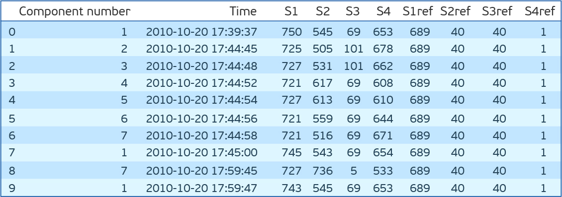
As you can see, there are seven components for each of which there are indications of four sensors, which are taken every 15 minutes. S1ref-S4ref in the description of the competition appear as reference values, but the values are very different from the sensor readings. In order not to waste time thinking about what they mean, we remove them. If you look at the distribution of values for each attribute (S1-S4), then it turns out that S1, S2 and S4 distributions are continuous, and S3 are discrete. In addition, if you look at the joint distribution of S2 and S4, it turns out that they are inversely proportional.
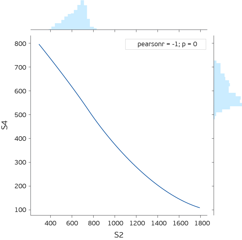
Although the deviation from the direct dependence may indicate an error, we will not check it, but simply remove S4.
Once again we will process a data set. We leave S1, S2 and S3. S1 and S2 are scaled by StandardScaler (we subtract the average and divide by the standard deviation), we translate S3 to OHE (One Hot Encoding). Stitch readings from all components of the installation in one line. Total 89 features. 2 * 7 = 14 - indications S1 and S2 for 7 components and 75 unique values of R3. Only 56 thousand of these lines.
Load the file with errors.
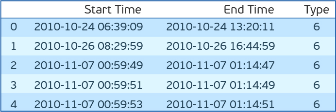
Before trying the listed algorithms on our data set, let me make one more small digression. It is necessary after all to be tested. For this, it is proposed to take the start time of the error and the end time. And all the readings inside this gap are considered abnormal, and outside - normal. There are many drawbacks to this approach. But especially one - abnormal behavior most likely occurs before the error is fixed. Shift for loyalty window anomaly half an hour ago in time. We will evaluate the F1-measure, accuracy (precision) and completeness (recall).
The code for selecting features and determining the quality of a model
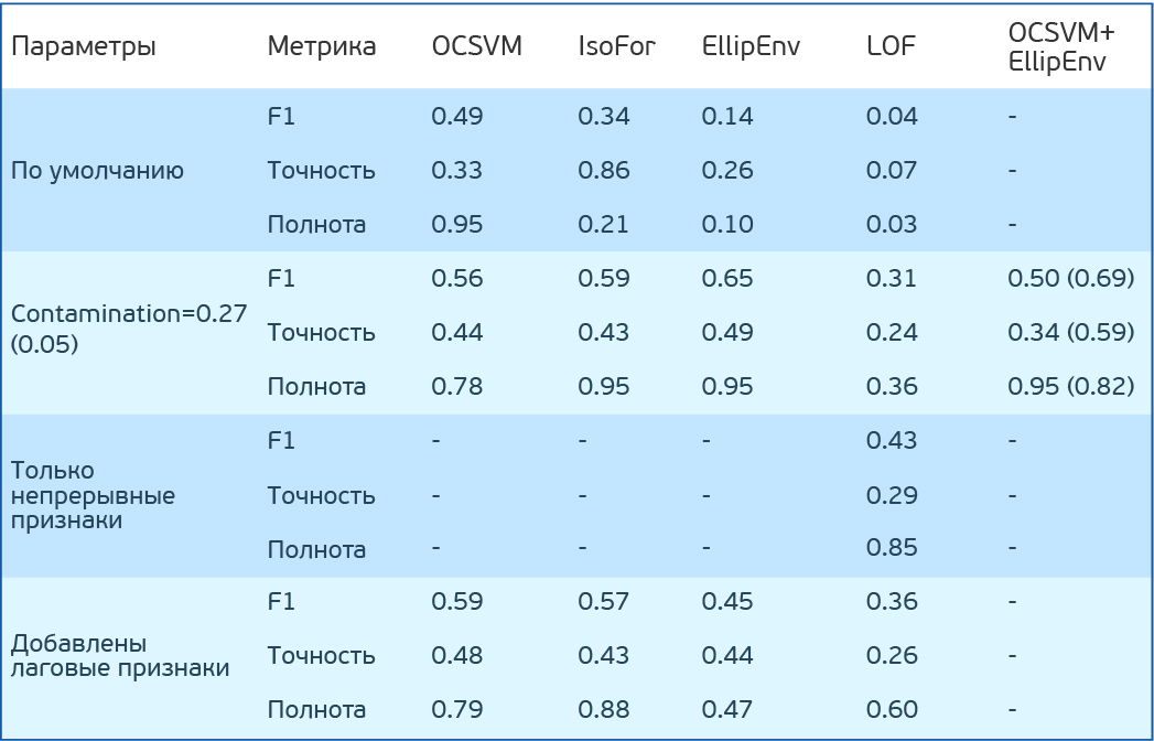 Test results of simple anomaly search algorithms in dataset PHM 2015 Data Challenge
Let's go back to the algorithms. Let's try One Class SVM (OCSVM), IsolationForest (IF), EllipticEnvelope (EE) and LocalOutlierFactor (LOF) on our data. To begin with, we will not set any parameters. I note that LOF can work in two modes. If novelty = False can only search for anomalies in the training sample (there is only fit_predict), if True, then it is aimed at finding anomalies outside the training sample (it can separately fit and predict). IF has a mode of (behavior) old and new. Use new. He gives better results.
OCSVM identifies anomalies well, but too many false-positive results. For other methods, the result is even worse.
But suppose we know the percentage of anomalies in the data. In our case, 27%. OCSVM has nu - the upper estimate for the percentage of errors and the lower one for the percentage of support vectors. The remaining methods of contamination - the percentage of errors in the data. In the IF and LOF methods, it is determined automatically, while for OCSVM and EE it is set to 0.1 by default. Let's try to set contamination (nu) to 0.27. Now the top result is at EE.
Code for checking models:
It is interesting to look at the distribution of anomalous indices for different methods. It can be seen that the LOF really works badly for this data. ITS has points that the algorithm considers extremely anomalous. However, there are normal points. In IsoFor and OCSVM, it is clear that the choice of a cut-off threshold (contamination / nu) is important, which will change the trade-off between accuracy and completeness.

It is logical that the readings of the sensors have a distribution close to normal, near stationary values. If we really have a marked test sample, and better still a validation sample, then contamination can be reset. Next is the question, what errors to focus more: false positive or false negative?
LOF result is very low. Not very impressive. But remember that at the entrance we have OHE variables along with the variables transformed by StandardScaler. And the default distance is Euclidean. But if you count only S1 and S2 variables, then the situation is corrected and the result is comparable with other methods. It is important, however, to understand that one of the key parameters of the listed metric classifiers is the number of neighbors. It significantly affects the quality, and it must be tune. The metric of distance itself would also be good to select.
Now we will try to combine the two models. At the beginning of one remove anomalies from the training set. And then we will train OCSVM on a cleaner learning set. According to the previous results, we observed the greatest completeness in EE. We clear the training set through EE, train OCSVM on it and get F1 = 0.50, Accuracy = 0.34, fullness = 0.95. Not impressive. But we set nu = 0.27. And our data is more or less “clean”. If we assume that the completeness of EE on the training sample will be the same, then 5% errors will remain. Let us set such nu and get F1 = 0.69, Accuracy = 0.59, completeness = 0.82. Fine. It is important to note that in other methods such a combination does not work, as they imply that the training sample and the test number of anomalies are the same. When teaching these methods on a pure training data set, contamination will have to be set less than in real data, and not close to zero, but it is better to select it for cross-validation.
It is interesting to look at the search result on the sequence of indications:

The figure shows a segment of the readings of the first and second sensors for 7 components. In the legend, the color of the corresponding errors (the beginning and end are shown by vertical lines of the same color). Dots indicate predictions: green - correct predictions, red - false positive, violet - false negative. The figure shows that it is difficult to visually determine the time of errors, and the algorithm copes with this task quite well. Although it is important to understand that the testimony of the third sensor is not given here. In addition, there are false-positive indications after the end of the error. Those. the algorithm sees that there are also erroneous values there, and we have marked this area as infallible. On the right in the figure, there is a visible area before the error, which we marked as erroneous (half an hour before the error), which is recognized as error-free, which leads to false-negative model errors. In the center of the picture is a coherent piece, recognized as an error. The conclusion can be drawn as follows: when solving the problem of searching for anomalies, it is necessary to interact closely with engineers who understand the essence of the systems, the output of which they need to be predicted, since checking the algorithms used on the markup does not fully reflect reality and does not simulate the conditions in which such algorithms could to be used.
Code for drawing graphics:
If the percentage of anomalies is below 5% and / or they are poorly separated from “normal” indicators, the methods listed above work poorly and it is worth using algorithms based on neural networks. In the simplest case, these will be:
Separately, it is worth noting the specifics of working with time series. It is important to understand that most of the above algorithms (except autoencoders and isolating forests) are likely to produce worse quality when adding lag tags (readings from previous times).
Let's try to add lag signs in our example. The description of the competition states that the values 3 hours before the error are not related to the error. Then add signs for 3 hours. Total 259 signs.
As a result, the OCSVM and IsolationForest results almost did not change, while the Elliptic Envelope and LOF fell.
To use information about the dynamics of the system, you should use auto-encoders with recurrent or convolutional neural networks. Or, for example, a combination of auto-coders, compressing information, and conventional approaches to search for anomalies based on compressed information. The opposite approach is also promising. The primary elimination of the most uncharacteristic points with standard algorithms, and then the training of the autoencoder is already on cleaner data.
 A source
There is a set of techniques for working with one-dimensional time series. All of them are aimed at predicting future readings, and the points that differ from the prediction are considered anomalies.
Triple exponential smoothing, decomposes the series into 3 components: level, trend and seasonality. Accordingly, if the series is presented in this form, the method works well. Facebook Prophet works on a similar principle, but the components themselves value differently. You can read more, for example, here .
In this method, the predictive model is based on autoregression and the moving average. If we are talking about expanding S (ARIMA), then we can also evaluate seasonality. Read more about the approach here , here and here .
When it comes to time series and there is information about the time of occurrence of errors, you can apply the methods of training with the teacher. In addition to the need for labeled data in this case, it is important to understand that predicting an error will depend on the nature of the error. If there are a lot of mistakes and different nature, then you will most likely need to predict each one individually, which will require even more marked data, but the prospects will be more attractive.
There are alternative ways to use machine learning in predictive service. For example, the prediction of system failure in the next N days (the task of classification). It is important to understand that such an approach requires that the occurrence of an error in the operation of the system be preceded by a period of degradation (not necessarily gradual). The most successful approach is the use of neural networks with convolutional and / or recurrent layers. Separately, it is worth noting the methods for augmentation of time series. The most interesting and at the same time simple for me are two approaches :
There is also a variant with the prediction of the remaining lifetime of the system (regression task). Here we can distinguish a separate approach: the prediction is not the life time, and the parameters of the Weibull distribution.
You can read about the distribution itself here , and here about using it in conjunction with recurrent meshes. This distribution has two parameters, α and β. α tells you when the event will occur, and β tells you how confident the algorithm is. Although the application of such an approach is promising, difficulties arise in learning the neural network in this case, since the algorithm is easier to be unsure at first than to predict an adequate lifetime.
Separately, it is worth noting the Cox regression . It allows you to predict the fault tolerance of the system for each point in time after the diagnosis, presenting it as a product of two functions. One function is a degradation of the system, independent of its parameters, i.e. common to any such systems. And the second is an exponential dependence on the parameters of a particular system. So for a person there is a common function associated with aging, more or less the same for all. But deterioration in health is also associated with the state of the internal organs, which is different for everyone.
I hope you now know a bit more about predictive service. I am sure you will have questions about the methods of machine learning, which are most often used for this technology. I will be happy to answer each of them in the comments. If you are interested in not just asking about what was written, but you want to do something similar, our team at CleverDATA is always happy to talented and enthusiastic professionals.
How popular is this approach in our country and in the West? The conclusion can be made, for example, under articles on Habré and in Medium. On Habré there are almost no articles on solving problems of predictive maintenance. On the Medium there is a whole set. Here, here and here it is well described, what are the goals and advantages of such an approach.
From this article you will learn:
')
- why do we need this technique
- which machine learning approaches are used more often for predictive maintenance,
- as I tried one of the techniques on a simple example.
What opportunities gives predictive service:
- controlled process of repair works, which are performed as needed, thus saving money, and without haste, which improves the quality of these works;
- identification of a specific equipment malfunction (the ability to purchase a specific part for replacement while the equipment is running offers tremendous advantages);
- optimization of equipment operation, loads, etc .;
- reducing the cost of regular equipment shutdown.
In the next article on Medium , the questions that need to be answered are well described in order to understand how to approach this question in a particular case.
When collecting data or choosing data for building a model, it is important to answer three groups of questions:
- Are all system problems predictable? Which predict is especially important?
- What is the failure process? Does the system stop working completely or does the mode of operation only change? Is this a quick process, instantaneous or gradual degradation?
- Is the system performance sufficiently reflecting its performance? Do they apply to individual parts of the system or to the system as a whole?
It is also important to understand in advance what you want to predict and what is possible to predict and what is not.
The article on Medium also lists questions that will help determine your specific goal:
- What to predict? Remaining lifetime, abnormal behavior or not, the likelihood of failing over the next N hours / days / weeks?
- Is there sufficient historical data?
- Whether it is known when the system produced anomalous readings, and when it did not. Is it possible to mark such indications?
- How far forward should the model see? How independent are the indications, reflecting the work of the system, in the interval of hours / day / week
- What needs to be optimized? Should the model catch as many violations as possible while giving a false alarm, or is it enough to catch several events without false alarms.
There is hope that the situation in the future will be corrected. So far, there are difficulties in the field of predictive maintenance: there are few examples of system malfunction, or there are enough time instants of system malfunction, but they are not marked; The failure process is unknown.
The main way to overcome difficulties in predictive service is to use anomaly search methods . Such algorithms do not require markup for training. For testing and debugging algorithms, markup is necessary in one form or another. Such methods are limited by the fact that they will not predict a specific breakdown, but only signal an abnormality of the indicators.
But this is not bad.
Methods
Now I want to talk about some of the features of anomaly detection approaches, and then together we will test the capabilities of some simple algorithms in practice.
Although for a particular situation, testing of several anomaly search algorithms and choosing the best one will be required, it is possible to determine some advantages and disadvantages of the main techniques used in this area.
First of all, it is important to understand in advance what percentage of anomalies are in the data.
If we are talking about the variation of the semi-supervised approach (we are learning only on “normal” data, and working (testing) then on data with anomalies), then the most optimal will be the choice of the one-class support vector method ( One-Class SVM ) . When using radial basis functions as a core, this algorithm builds a nonlinear surface around the origin. The cleaner the training data, the better it works.
In other cases, the need to know the ratio of anomalous and "normal" points also remains - to determine the cut-off threshold.
If the number of anomalies in the data is more than 5%, and they are quite well separated from the main sample, you can use the standard methods of searching for anomalies.
In this case, the most stable in terms of quality is the isolation forest method ( isolation forest ) : the data are split randomly. A more characteristic reading is more likely to get deeper, while unusual indicators will be separated from the rest of the sample in the first iterations.
The rest of the algorithms work better if they “fit” the specifics of the data.
When the data has a normal distribution, the Elliptic envelope method is suitable, approximating the data with a multidimensional normal distribution. The less likely that the point belongs to the distribution, the greater the likelihood that it is anomalous.
If the data is presented in such a way that the relative position of different points reflects their differences well, then metric methods are good choices: for example, k nearest neighbors, kth nearest neighbor, ABOD (angle-based outlier detection) or LOF (local outlier factor) ) .
All these methods assume that the “right” indicators are concentrated in one area of multidimensional space. If among the k (or kth) nearest neighbors everything is far from the target, then the point is an anomaly. For ABOD, the reasoning is similar: if all k nearest points are in the same sector of the space relative to the considered one, then the point is an anomaly. For LOF: if the local density (predetermined for each point by k nearest neighbors) is lower than that of k nearest neighbors, then the point is an anomaly.
If the data is well clustered, methods based on cluster analysis are a good choice. If the point is equidistant from the centers of several clusters, then it is anomalous.
If the directions of the largest change in the dispersion are well distinguished in the data, then it seems to be a good choice - search for anomalies based on the principal component method . In this case, deviations from the mean value for n1 (the most “main” components) and for n2 (the least “main”) are considered as a measure of anomaly.
For example, it is proposed to look at the data set from The Prognostics and Health Management Society (PHM Society) . This non-profit organization organizes competitions every year. In 2018, for example, it was required to predict errors in operation and the time to failure of an ion beam etching installation . We will take the data set for 2015 . It shows the readings of several sensors for 30 installations (training sample), and it is required to predict when and what error will occur.
I did not find answers on the test sample in the network, so we will only play with the training one.
In general, all installations are similar, but differ, for example, in the number of components, in the number of anomalies, etc. Therefore, to study at the first 20, and test - for others does not make much sense.
So, choose one of the installations, load it and take a look at this data. The article will not be about feature engineering , so we will not peer hard.
import pandas as pd import matplotlib.pyplot as plt %matplotlib inline import seaborn as sns from sklearn.covariance import EllipticEnvelope from sklearn.neighbors import LocalOutlierFactor from sklearn.ensemble import IsolationForest from sklearn.svm import OneClassSVM dfa=pd.read_csv('plant_12a.csv',names=['Component number','Time','S1','S2','S3','S4','S1ref','S2ref','S3ref','S4ref']) dfa.head(10) As you can see, there are seven components for each of which there are indications of four sensors, which are taken every 15 minutes. S1ref-S4ref in the description of the competition appear as reference values, but the values are very different from the sensor readings. In order not to waste time thinking about what they mean, we remove them. If you look at the distribution of values for each attribute (S1-S4), then it turns out that S1, S2 and S4 distributions are continuous, and S3 are discrete. In addition, if you look at the joint distribution of S2 and S4, it turns out that they are inversely proportional.
Although the deviation from the direct dependence may indicate an error, we will not check it, but simply remove S4.
Once again we will process a data set. We leave S1, S2 and S3. S1 and S2 are scaled by StandardScaler (we subtract the average and divide by the standard deviation), we translate S3 to OHE (One Hot Encoding). Stitch readings from all components of the installation in one line. Total 89 features. 2 * 7 = 14 - indications S1 and S2 for 7 components and 75 unique values of R3. Only 56 thousand of these lines.
Load the file with errors.
dfc=pd.read_csv('plant_12c.csv',names=['Start Time', 'End Time','Type']) dfc.head() Before trying the listed algorithms on our data set, let me make one more small digression. It is necessary after all to be tested. For this, it is proposed to take the start time of the error and the end time. And all the readings inside this gap are considered abnormal, and outside - normal. There are many drawbacks to this approach. But especially one - abnormal behavior most likely occurs before the error is fixed. Shift for loyalty window anomaly half an hour ago in time. We will evaluate the F1-measure, accuracy (precision) and completeness (recall).
The code for selecting features and determining the quality of a model
def load_and_preprocess(plant_num): # , dfa=pd.read_csv('plant_{}a.csv'.format(plant_num),names=['Component number','Time','S1','S2','S3','S4','S1ref','S2ref','S3ref','S4ref']) dfc=pd.read_csv('plant_{}c.csv'.format(plant_num),names=['Start Time','End Time','Type']).drop(0,axis=0) N_comp=len(dfa['Component number'].unique()) # 15 dfa['Time']=pd.to_datetime(dfa['Time']).dt.round('15min') # 6 ( , ) dfc=dfc[dfc['Type']!=6] dfc['Start Time']=pd.to_datetime(dfc['Start Time']) dfc['End Time']=pd.to_datetime(dfc['End Time']) # , OHE 3- dfa=pd.concat([dfa.groupby('Time').nth(i)[['S1','S2','S3']].rename(columns={"S1":"S1_{}".format(i),"S2":"S2_{}".format(i),"S3":"S3_{}".format(i)}) for i in range(N_comp)],axis=1).dropna().reset_index() for k in range(N_comp): dfa=pd.concat([dfa.drop('S3_'+str(k),axis=1),pd.get_dummies(dfa['S3_'+str(k)],prefix='S3_'+str(k))],axis=1).reset_index(drop=True) # df_train,df_test=train_test_split(dfa,test_size=0.25,shuffle=False) cols_to_scale=df_train.filter(regex='S[1,2]').columns scaler=preprocessing.StandardScaler().fit(df_train[cols_to_scale]) df_train[cols_to_scale]=scaler.transform(df_train[cols_to_scale]) df_test[cols_to_scale]=scaler.transform(df_test[cols_to_scale]) return df_train,df_test,dfc # def get_true_labels(measure_times,dfc,shift_delta): idxSet=set() dfc['Start Time']-=pd.Timedelta(minutes=shift_delta) dfc['End Time']-=pd.Timedelta(minutes=shift_delta) for idx,mes_time in tqdm_notebook(enumerate(measure_times),total=measure_times.shape[0]): intersect=np.array(dfc['Start Time']<mes_time).astype(int)*np.array(dfc['End Time']>mes_time).astype(int) idxs=np.where(intersect)[0] if idxs.shape[0]: idxSet.add(idx) dfc['Start Time']+=pd.Timedelta(minutes=shift_delta) dfc['End Time']+=pd.Timedelta(minutes=shift_delta) true_labels=pd.Series(index=measure_times.index) true_labels.iloc[list(idxSet)]=1 true_labels.fillna(0,inplace=True) return true_labels # def check_model(model,df_train,df_test,filt='S[123]'): model.fit(df_train.drop('Time',axis=1).filter(regex=(filt))) y_preds = pd.Series(model.predict(df_test.drop(['Time','Label'],axis=1).filter(regex=(filt)))).map({-1:1,1:0}) print('F1 score: {:.3f}'.format(f1_score(df_test['Label'],y_preds))) print('Precision score: {:.3f}'.format(precision_score(df_test['Label'],y_preds))) print('Recall score: {:.3f}'.format(recall_score(df_test['Label'],y_preds))) score = model.decision_function(df_test.drop(['Time','Label'],axis=1).filter(regex=(filt))) sns.distplot(score[df_test['Label']==0]) sns.distplot(score[df_test['Label']==1]) df_train,df_test,anomaly_times=load_and_preprocess(12) df_test['Label']=get_true_labels(df_test['Time'],dfc,30) Let's go back to the algorithms. Let's try One Class SVM (OCSVM), IsolationForest (IF), EllipticEnvelope (EE) and LocalOutlierFactor (LOF) on our data. To begin with, we will not set any parameters. I note that LOF can work in two modes. If novelty = False can only search for anomalies in the training sample (there is only fit_predict), if True, then it is aimed at finding anomalies outside the training sample (it can separately fit and predict). IF has a mode of (behavior) old and new. Use new. He gives better results.
OCSVM identifies anomalies well, but too many false-positive results. For other methods, the result is even worse.
But suppose we know the percentage of anomalies in the data. In our case, 27%. OCSVM has nu - the upper estimate for the percentage of errors and the lower one for the percentage of support vectors. The remaining methods of contamination - the percentage of errors in the data. In the IF and LOF methods, it is determined automatically, while for OCSVM and EE it is set to 0.1 by default. Let's try to set contamination (nu) to 0.27. Now the top result is at EE.
Code for checking models:
def check_model(model,df_train,df_test,filt='S[123]'): model_type,model = model model.fit(df_train.drop('Time',axis=1).filter(regex=(filt))) y_preds = pd.Series(model.predict(df_test.drop(['Time','Label'],axis=1).filter(regex=(filt)))).map({-1:1,1:0}) print('F1 score for {}: {:.3f}'.format(model_type,f1_score(df_test['Label'],y_preds))) print('Precision score for {}: {:.3f}'.format(model_type,precision_score(df_test['Label'],y_preds))) print('Recall score for {}: {:.3f}'.format(model_type,recall_score(df_test['Label'],y_preds))) score = model.decision_function(df_test.drop(['Time','Label'],axis=1).filter(regex=(filt))) sns.distplot(score[df_test['Label']==0]) sns.distplot(score[df_test['Label']==1]) plt.title('Decision score distribution for {}'.format(model_type)) plt.show() It is interesting to look at the distribution of anomalous indices for different methods. It can be seen that the LOF really works badly for this data. ITS has points that the algorithm considers extremely anomalous. However, there are normal points. In IsoFor and OCSVM, it is clear that the choice of a cut-off threshold (contamination / nu) is important, which will change the trade-off between accuracy and completeness.
It is logical that the readings of the sensors have a distribution close to normal, near stationary values. If we really have a marked test sample, and better still a validation sample, then contamination can be reset. Next is the question, what errors to focus more: false positive or false negative?
LOF result is very low. Not very impressive. But remember that at the entrance we have OHE variables along with the variables transformed by StandardScaler. And the default distance is Euclidean. But if you count only S1 and S2 variables, then the situation is corrected and the result is comparable with other methods. It is important, however, to understand that one of the key parameters of the listed metric classifiers is the number of neighbors. It significantly affects the quality, and it must be tune. The metric of distance itself would also be good to select.
Now we will try to combine the two models. At the beginning of one remove anomalies from the training set. And then we will train OCSVM on a cleaner learning set. According to the previous results, we observed the greatest completeness in EE. We clear the training set through EE, train OCSVM on it and get F1 = 0.50, Accuracy = 0.34, fullness = 0.95. Not impressive. But we set nu = 0.27. And our data is more or less “clean”. If we assume that the completeness of EE on the training sample will be the same, then 5% errors will remain. Let us set such nu and get F1 = 0.69, Accuracy = 0.59, completeness = 0.82. Fine. It is important to note that in other methods such a combination does not work, as they imply that the training sample and the test number of anomalies are the same. When teaching these methods on a pure training data set, contamination will have to be set less than in real data, and not close to zero, but it is better to select it for cross-validation.
It is interesting to look at the search result on the sequence of indications:
The figure shows a segment of the readings of the first and second sensors for 7 components. In the legend, the color of the corresponding errors (the beginning and end are shown by vertical lines of the same color). Dots indicate predictions: green - correct predictions, red - false positive, violet - false negative. The figure shows that it is difficult to visually determine the time of errors, and the algorithm copes with this task quite well. Although it is important to understand that the testimony of the third sensor is not given here. In addition, there are false-positive indications after the end of the error. Those. the algorithm sees that there are also erroneous values there, and we have marked this area as infallible. On the right in the figure, there is a visible area before the error, which we marked as erroneous (half an hour before the error), which is recognized as error-free, which leads to false-negative model errors. In the center of the picture is a coherent piece, recognized as an error. The conclusion can be drawn as follows: when solving the problem of searching for anomalies, it is necessary to interact closely with engineers who understand the essence of the systems, the output of which they need to be predicted, since checking the algorithms used on the markup does not fully reflect reality and does not simulate the conditions in which such algorithms could to be used.
Code for drawing graphics:
def plot_time_course(df_test,dfc,y_preds,start,end,vert_shift=4): plt.figure(figsize=(15,10)) cols=df_train.filter(regex=('S[12]')).columns add=0 preds_idx=y_preds.iloc[start:end][y_preds[0]==1].index true_idx=df_test.iloc[start:end,:][df_test['Label']==1].index tp_idx=set(true_idx.values).intersection(set(preds_idx.values)) fn_idx=set(true_idx.values).difference(set(preds_idx.values)) fp_idx=set(preds_idx.values).difference(set(true_idx.values)) xtime=df_test['Time'].iloc[start:end] for col in cols: plt.plot(xtime,df_test[col].iloc[start:end]+add) plt.scatter(xtime.loc[tp_idx].values,df_test.loc[tp_idx,col]+add,color='green') plt.scatter(xtime.loc[fn_idx].values,df_test.loc[fn_idx,col]+add,color='violet') plt.scatter(xtime.loc[fp_idx].values,df_test.loc[fp_idx,col]+add,color='red') add+=vert_shift failures=dfc[(dfc['Start Time']>xtime.iloc[0])&(dfc['Start Time']<xtime.iloc[-1])] unique_fails=np.sort(failures['Type'].unique()) colors=np.array([np.random.rand(3) for fail in unique_fails]) for fail_idx in failures.index: c=colors[np.where(unique_fails==failures.loc[fail_idx,'Type'])[0]][0] plt.axvline(failures.loc[fail_idx,'Start Time'],color=c) plt.axvline(failures.loc[fail_idx,'End Time'],color=c) leg=plt.legend(unique_fails) for i in range(len(unique_fails)): leg.legendHandles[i].set_color(colors[i]) If the percentage of anomalies is below 5% and / or they are poorly separated from “normal” indicators, the methods listed above work poorly and it is worth using algorithms based on neural networks. In the simplest case, these will be:
- autoencoders (high error of a trained autoencoder will signal anomalous readings);
- recurrent networks (learns by sequence to predict the last reading. If the difference is large, the point is anomalous).
Separately, it is worth noting the specifics of working with time series. It is important to understand that most of the above algorithms (except autoencoders and isolating forests) are likely to produce worse quality when adding lag tags (readings from previous times).
Let's try to add lag signs in our example. The description of the competition states that the values 3 hours before the error are not related to the error. Then add signs for 3 hours. Total 259 signs.
As a result, the OCSVM and IsolationForest results almost did not change, while the Elliptic Envelope and LOF fell.
To use information about the dynamics of the system, you should use auto-encoders with recurrent or convolutional neural networks. Or, for example, a combination of auto-coders, compressing information, and conventional approaches to search for anomalies based on compressed information. The opposite approach is also promising. The primary elimination of the most uncharacteristic points with standard algorithms, and then the training of the autoencoder is already on cleaner data.
There is a set of techniques for working with one-dimensional time series. All of them are aimed at predicting future readings, and the points that differ from the prediction are considered anomalies.
Holt-Winters Model
Triple exponential smoothing, decomposes the series into 3 components: level, trend and seasonality. Accordingly, if the series is presented in this form, the method works well. Facebook Prophet works on a similar principle, but the components themselves value differently. You can read more, for example, here .
S (ARIMA)
In this method, the predictive model is based on autoregression and the moving average. If we are talking about expanding S (ARIMA), then we can also evaluate seasonality. Read more about the approach here , here and here .
Other Predictive Service Approaches
When it comes to time series and there is information about the time of occurrence of errors, you can apply the methods of training with the teacher. In addition to the need for labeled data in this case, it is important to understand that predicting an error will depend on the nature of the error. If there are a lot of mistakes and different nature, then you will most likely need to predict each one individually, which will require even more marked data, but the prospects will be more attractive.
There are alternative ways to use machine learning in predictive service. For example, the prediction of system failure in the next N days (the task of classification). It is important to understand that such an approach requires that the occurrence of an error in the operation of the system be preceded by a period of degradation (not necessarily gradual). The most successful approach is the use of neural networks with convolutional and / or recurrent layers. Separately, it is worth noting the methods for augmentation of time series. The most interesting and at the same time simple for me are two approaches :
- selects the continuous part of the series (for example, 70%, and the rest is removed) and stretches to its original size
- the continuous part of the series is selected (for example, 20%) and stretched or compressed. After that, the entire row is respectively compressed or stretched to its original size.
There is also a variant with the prediction of the remaining lifetime of the system (regression task). Here we can distinguish a separate approach: the prediction is not the life time, and the parameters of the Weibull distribution.
You can read about the distribution itself here , and here about using it in conjunction with recurrent meshes. This distribution has two parameters, α and β. α tells you when the event will occur, and β tells you how confident the algorithm is. Although the application of such an approach is promising, difficulties arise in learning the neural network in this case, since the algorithm is easier to be unsure at first than to predict an adequate lifetime.
Separately, it is worth noting the Cox regression . It allows you to predict the fault tolerance of the system for each point in time after the diagnosis, presenting it as a product of two functions. One function is a degradation of the system, independent of its parameters, i.e. common to any such systems. And the second is an exponential dependence on the parameters of a particular system. So for a person there is a common function associated with aging, more or less the same for all. But deterioration in health is also associated with the state of the internal organs, which is different for everyone.
I hope you now know a bit more about predictive service. I am sure you will have questions about the methods of machine learning, which are most often used for this technology. I will be happy to answer each of them in the comments. If you are interested in not just asking about what was written, but you want to do something similar, our team at CleverDATA is always happy to talented and enthusiastic professionals.
Are there any vacancies? Of course!
Source: https://habr.com/ru/post/447190/
All Articles