Modeling the MUSIC algorithm for determining the direction of arrival of an electromagnetic wave

aaspcats

Foreword

I will begin my entry from afar. Long ago, in the distant 2016-2017 years, your humble servant managed to go on a semi-annual training to the distant city of Ilmenau (Germany), where he successfully (in general) finished the master program in Communications and Signal processing . The program was not easy, but now it’s pleasant to remember about it. Sometimes...

So, at the end of this training, besides a diploma, I had quite a lot of different materials left on my hands, which seemed to me to be wrong not to share.

One of these materials is in front of you.

What goals did I pursue while I was preparing a seminar :

talk about some of the already well-established, “smart” approaches to the topic of antenna arrays most accessible and do it in Russian;
conduct a small simulation in Python 3 , in order to persuade fellow radio engineers to look at programming languages (if you haven't looked closely);
to give references to good English-language literature - without reading foreign sources, now, alas, nowhere.

What we consider :

The MUSIC (MUltiple SIgnal Classification) method is, in fact, a reference to the preview.

An example of diagramming and the MVDR method can be found by reference (if there are questions or suggestions for additional material, then the discussion can be continued on Github.Gist).

As I said above, we will use Python, as follows:

import numpy as np import matplotlib.pyplot as plt

Why not MATLAB, one of the most popular and convenient candidates for modeling using linear algebra, you ask? Because, I want to show that this work can be done in Python, and the scope of Python is much broader than that of MATLAB. Therefore, to be familiar with the Python syntax is a good thing, in my opinion.

Let's start!

Formulas are prepared via https://upmath.me/ . Thanks to the creators for a great tool!

Formulation of the problem

Suppose there is a linear antenna array consisting of a number of elements spaced apart from each other. $\ Delta = \ frac {\ lambda} {2}$ (antenna array pitch) where $\ lambda$ - the length of the carrier electromagnetic (EM) wave.

Electromagnetic waves fall on this antenna array from different directions.

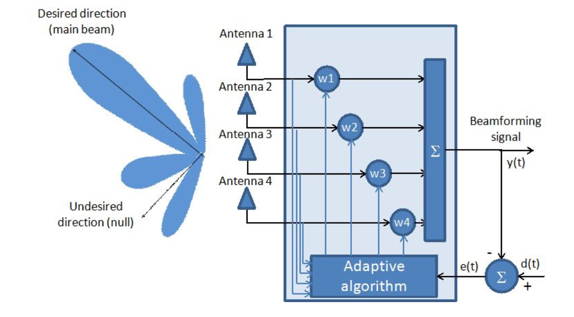
Fig. 1. Adaptive antenna system.

As can be seen from the figure, the antenna array is considered as an adaptive filter.

In fact, finding the optimal vector of coefficients ( $\ mathbf {w} _ {opt}$ ) and is the main task of adaptive antenna arrays from a mathematical point of view.

Initially, we do not know exactly from which directions the signals come and how many of them. It is to resolve this contradiction that we will apply the MUSIC algorithm — an algorithm for estimating spatial frequencies with high resolution.

Simulation of the received signal

The model of the received signal we can present through the formula:

$\ mathbf {X} = \ mathbf {A} \ mathbf {S} + \ mathbf {N}$

Where $\ mathbf {A} = [\ mathbf {a} (\ theta_1) \ quad \ mathbf {a} (\ theta_2) \ quad ... \ quad \ mathbf {a} (\ theta_d)]$ - matrix of scanning vectors (steering vectors) of the antenna array ( $a_i = \ exp (-j \ mu m_i)$ , m = 0, 1 ... (M-1) , - the number of elements of the antenna array, - the number of sources of EM waves, $\ theta$ - angle of arrival of the EM wave), $\ mathbf {s}$ - matrix of transmitted characters, and $\ mathbf {N}$ - matrix of additive noise.

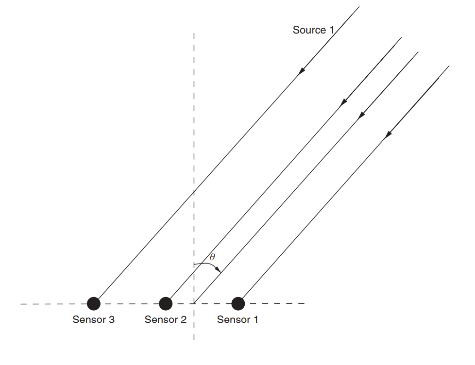
Fig. 2. Non-directional linear antenna array (ULAA - uniform linear anntenna array) [1, p. 32].

We rethink this formula in the “everyday” way: we get some “porridge” from various signals on our lattice, which we denote by $\ mathbf {X}$ . We do not explicitly receive information on the number of sources and directions, however, information about this is still contained in the received signal.

Begin to look!

To do this, they usually proceed to manipulations not with the matrices of the complex amplitudes of the signals, but with their covariances (that is, with the powers):

$\ mathbf {R} _ {xx} = \ mathbf {X} \ mathbf {X} ^ H = \ mathbf {A} \ mathbf {R} _ {ss} \ mathbf {A} ^ H + \ mathbf {R} _ {nn}$

Conditions

Let us introduce an important condition for consideration: Rayleigh angle resolution limit:

$sin (\ theta_R) = \ frac {\ lambda} {D}$

Where $D = M \ Delta$ Is the length of the linear lattice.

Let's redefine the angle of arrival of an electromagnetic wave through the concept of spatial frequency:

$\ mu_R = \ frac {2 \ pi} {\ lambda} \ Delta sin (\ theta_R) = \ frac {2 \ pi} {\ lambda} \ Delta \ frac {\ lambda} {\ Delta M} = \ frac { 2 \ pi} {M}$

Where $\ mu_R$ - there is a standard width of the main lobe of the DN ( standard beam width ).

To check how effective our method is and under what conditions, we introduce some set values for the angular separation:

$\ mu_1 = - \ mu_R, \ quad \ mu_2 = 0, \ quad \ mu_3 = \ mu_R \ quad$ - separation in one beam width;
$\ mu_1 = -0.5 \ mu_R, \ quad \ mu_2 = 0, \ quad \ mu_3 = 0.5 \ mu_R \ quad$ - division into one second beam width;
$\ mu_1 = -0.3 \ mu_R, \ quad \ mu_2 = 0, \ quad \ mu_3 = 0.3 \ mu_R \ quad$ - separation of three tenths of the beam width.

Define input parameters:

 M = 10 #    () SNR = 10 #  - (dB) d = 3 #     N = 50 #  "" (snapshots) S = ( np.sign(np.random.randn(d,N)) + 1j * np.sign(np.random.randn(d,N)) ) / np.sqrt(2) # QPSK W = ( np.random.randn(M,N) + 1j * np.random.randn(M,N) ) / np.sqrt(2) * 10**(-SNR/20) # AWGN #  : # sqrt(N0/2)*(G1 + jG2), #  G1  G2 -   . # .. Es( )  QPSK  1 ,    (noise spectral density): # N0 = (Es/N)^(-1) = SNR^(-1) [] (   ,  SNR = Es/N0); #    : # SNR_dB = 10log10(SNR) => N0_dB = -10log10(SNR) = -SNR_dB []; #    SNR    (..  ),   : # SNR = 10^(SNR_dB/10) => sqrt(N0) = (10^(-SNR_dB/10))^(1/2) = 10^(-SNR_dB/20) mu_R = 2*np.pi / M

A bit of theory about the method itself.

First of all, we note that the progenitor of the MUSIC method is the Pisarenko method (1973). The considered problem of the Pisarenko method was to estimate the frequencies of the sum of complex exponentials in white noise. VF Pisarenko demonstrated that frequencies can be found from the eigenvectors corresponding to the minimum eigenvalue of the autocorrelation matrix. Subsequently, this method became a special case of the MUSIC method. [2, c. 459]

Schmidt and his colleagues proposed the Multiple Signal Classification Algorithm (MUSIC) in 1979 [4]. The main approach of this algorithm is the decomposition of the covariance matrix of the received signal into eigenvalues. Since this algorithm takes into account uncorrelated noise, the generated covariance matrix has a diagonal form. Here, the signal and noise subspaces are calculated using linear algebra, and are orthogonal to each other. Therefore, the algorithm uses the orthogonality property to separate signal and noise subspaces [5].

The generalized MUSIC algorithm can be defined as follows:

Find the covariance matrix $\ mathbf {R} _ {xx}$
Find eigenvectors via EVD or another suitable numerical algorithm:

$\ mathbf {R} _ {xx} = \ mathbf {U} \ mathbf {\ Lambda} \ mathbf {U} ^ H \ qquad (1)$

Find the pseudospectrum (why with the pseudo prefix, we will discuss below) MUSIC using the following formula:

$P_ {MU} (e ^ {j \ omega}) = \ frac {1} {\ sum \ limits_ {i = d + 1} ^ {M} | \ mathbf {a} ^ H \ mathbf {u} _i | ^ 2} \ qquad (2)$

Where $\ mathbf {a} = \ begin {bmatrix} e ^ {j0 \ omega} & e ^ {j1 \ omega} & e ^ {j2 \ omega} & ... & e ^ {j (M-1) \ omega } \ end {bmatrix} ^ T$ - vector of exponentials for the frequency ω, lying in a certain specified range, and $\ mathbf {u} _i$ - i-th eigenvector (eigen vector) of the covariance matrix (1), corresponding to the noise subspace of the matrix (1) - hence the indexation with d + 1 ( - rank of the matrix (1)).

For greater clarity, try to run the corresponding MATLAB script presented by reference . Pay attention to two main points:
instead of calculating the square of the second norm in the denominator (2), the authors apply the FFT algorithm to the eigenvectors, which facilitates modeling due to the use of built-in functions and, in general, does not contradict the theory from a mathematical point of view;
the calculation of the covariance matrix is performed through convolutional matrices; a different approach was shown above for estimating spatial frequencies.

As you might guess from the name, MUSIC is also a classic method for estimating the direction of reception with high resolution. The algorithm for calculating pseudospectra in this context is given below:

find the covariance matrix of the received signal;
find the zero subspace $\ mathbf {U} _0$ :

$\ mathbf {U} = [\ mathbf {U} _s \ quad \ mathbf {U} _0]$

choose some search range:

$a (\ mu) = \ begin {bmatrix} e ^ {j0 \ mu_1} & ... & e ^ {j0 \ mu_Q} \\ ... & ... & ... \\ e ^ {j ( M-1) \ mu_1} & ... & e ^ {j (M-1) \ mu_Q} \ end {bmatrix}$

Where $\ mu = - \ frac {2 \ pi f_c} {c} \ Delta sin \ theta = - \ frac {2 \ pi} {\ lambda} \ Delta sin \ theta$

calculate the pseudospectrum:

$P_ {MU} (\ theta) = \ frac {\ mathbf {a} ^ H (\ theta) \ mathbf {a} (\ theta)} {\ mathbf {a} ^ H (\ theta) \ mathbf {U} _0 \ mathbf {U} _0 ^ H \ mathbf {a} (\ theta)}$

The relationship between spectral analysis and arrival angle analysis (DoA - direction of arriaval) of EM waves is described in Table 1.

Table 1 Relationship between MUSIC applications : Signal array processing and Harmonic search [6].

Variable	Signal array processing	Harmonic search
	Number of sensors	The number of time periods
	The number of time periods	The number of experiments
	The number of wave fronts	The number of complex components
$\ mu$	Spatial frequencies	Normalized frequencies

In general, the process of receiving through arrays (lattices) can be compared with the process of classical discretization, since in essence, each sensor, taking a wave with a certain phase delay (i.e. with a certain time delay), performs the functions of a sampling delta pulse. The number of realizations (experiments) of the classical spectral analysis will correspond to the number of time periods (snapshots). Each source will have its own wavefront, which is equivalent to the number of unique sinusoids of the signal in the case of spectral analysis.

Now back to the moment of calculating the eigenvectors. We already mentioned above that the vectors $a (\ theta_i) \ epsilon A$ where i = 1,2, .., d orthogonal to the noise subspace of the covariance matrix, i.e .:

$a (\ theta_i) ^ TU_0 = 0 ^ T$

As a matter of fact, we see a system of equations, solving which we can find the roots - eigenvectors. Such a method, in contrast to numerical algorithms (to which, as we noted above, EVD applies), allows one to obtain real, rather than approximate, eigenvalues. That is why this approach allows to obtain not a pseudospectrum, but a spectrum. The same idea formed the basis of the Root MUSIC algorithm.

Modeling

Phew! Finally, all the formulas are described and explained to some extent. We can start modeling.

 cases = [[-1., 0, 1.], [-0.5, 0, 0.5], [-0.3, 0, 0.3],] for idxm, c in enumerate(cases): #   ( ): mu_1 = c[0]*mu_R mu_2 = c[1]*mu_R mu_3 = c[2]*mu_R #   a_1 = np.exp(1j*mu_1*np.arange(M)) a_2 = np.exp(1j*mu_2*np.arange(M)) a_3 = np.exp(1j*mu_3*np.arange(M)) A = (np.array([a_1, a_2, a_3])).T #    X = np.dot(A,S) + W #    R = np.dot(X,np.matrix(X).H) U, Sigma, Vh = np.linalg.svd(X, full_matrices=True) U_0 = U[:,d:] #   thetas = np.arange(-90,91)*(np.pi/180) #   mus = np.pi*np.sin(thetas) #    a = np.empty((M, len(thetas)), dtype = complex) for idx, mu in enumerate(mus): a[:,idx] = np.exp(1j*mu*np.arange(M)) # MVDR: S_MVDR = np.empty(len(thetas), dtype = complex) for idx in range(np.shape(a)[1]): a_idx = (a[:, idx]).reshape((M, 1)) S_MVDR[idx] = 1 / (np.dot(np.matrix(a_idx).H, np.dot(np.linalg.pinv(R),a_idx))) # MUSIC: S_MUSIC = np.empty(len(thetas), dtype = complex) for idx in range(np.shape(a)[1]): a_idx = (a[:, idx]).reshape((M, 1)) S_MUSIC[idx] = np.dot(np.matrix(a_idx).H,a_idx)\ / (np.dot(np.matrix(a_idx).H, np.dot(U_0,np.dot(np.matrix(U_0).H,a_idx)))) plt.subplots(figsize=(10, 5), dpi=150) plt.semilogy(thetas*(180/np.pi), np.real( (S_MVDR / max(S_MVDR))), color='green', label='MVDR') plt.semilogy(thetas*(180/np.pi), np.real((S_MUSIC/ max(S_MUSIC))), color='red', label='MUSIC') plt.grid(color='r', linestyle='-', linewidth=0.2) plt.xlabel('Azimuth angles θ (degrees)') plt.ylabel('Power (pseudo)spectrum (normalized)') plt.legend() plt.title('Case #'+str(idxm+1)) plt.show()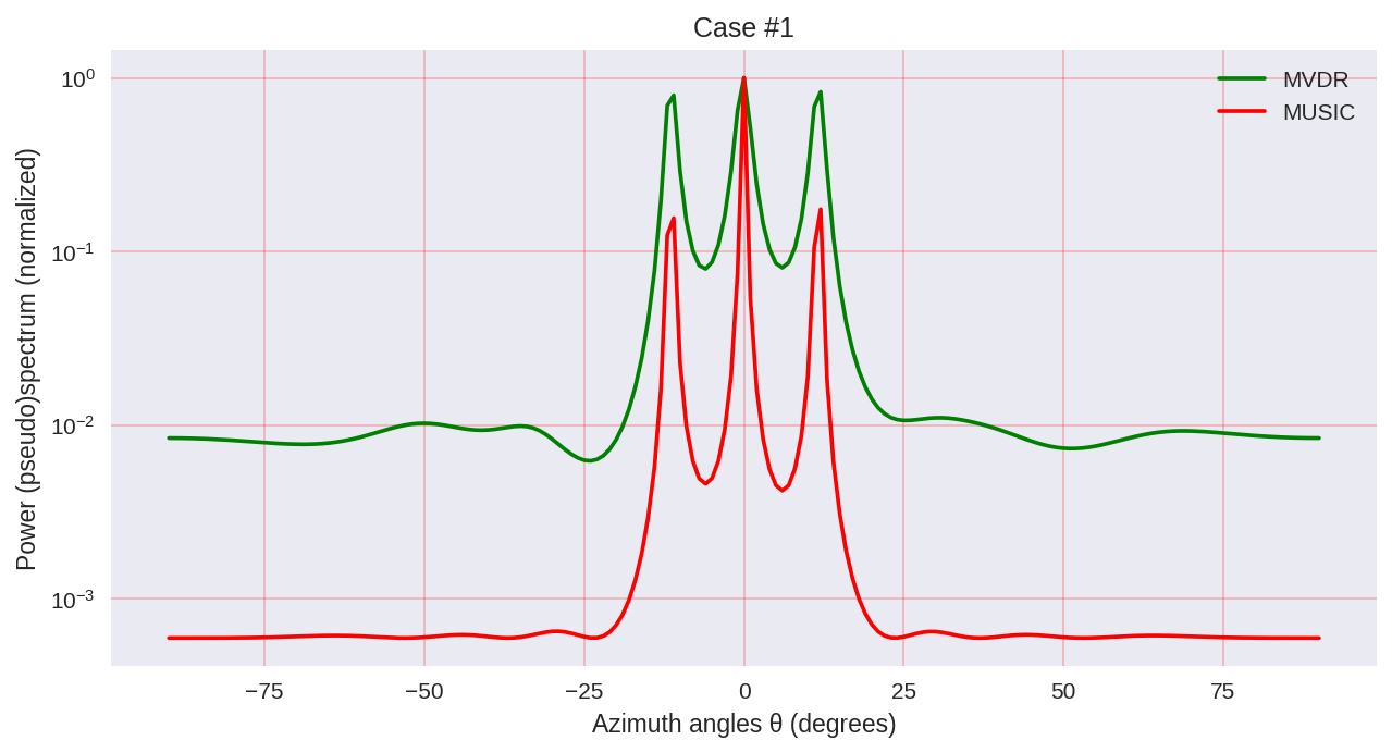

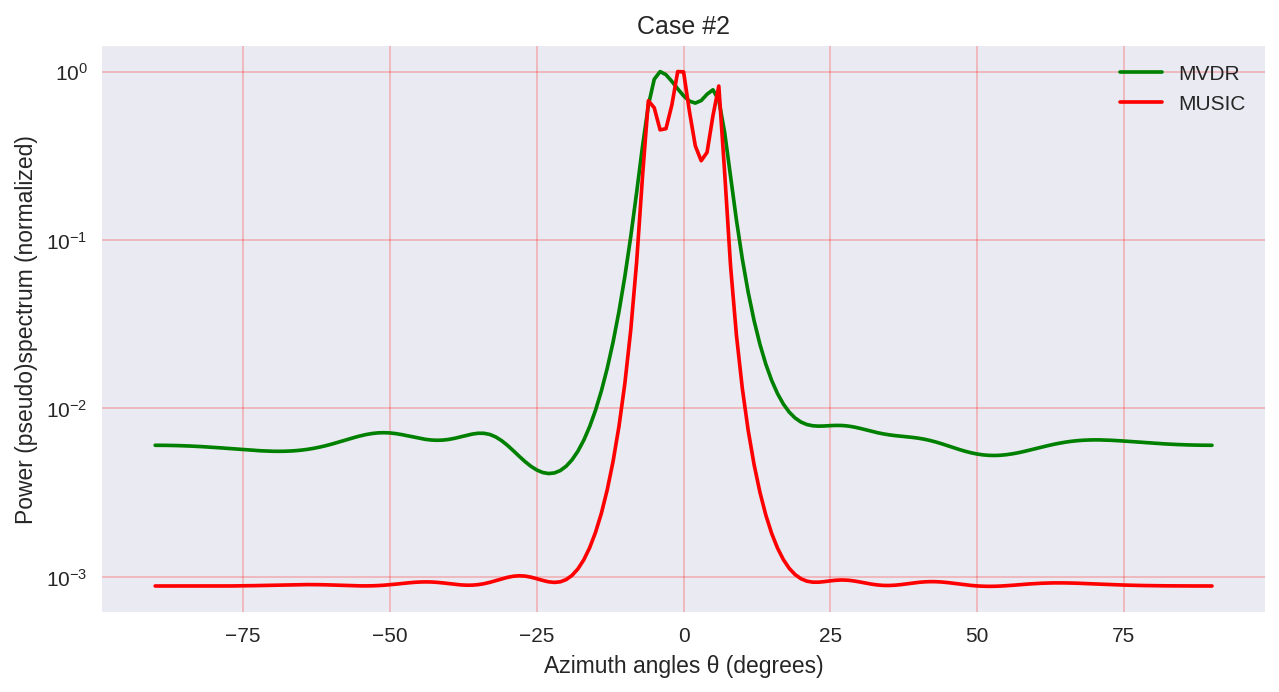
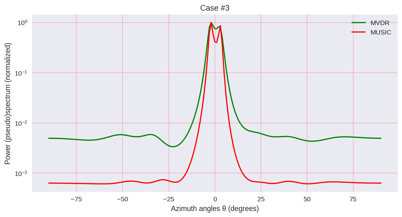
As we can see, MUSIC has a higher resolution and allows to achieve, in general, better results than, for example, MVDR allows - the same representative of parametric methods of spectral analysis.

However, it should be borne in mind that when using MUSIC, we use more computationally more expensive algorithms, such as EVD or SVD, which is some price for greater accuracy.

So it goes.

References:

Haykin, Simon, and KJ Ray Liu. Handbook on array processing and sensor networks. Vol. 63. John Wiley & Sons, 2010. pp. 102-107
Hayes MH Statistical digital processing and modeling. - John Wiley & Sons, 2009.
Haykin, Simon S. Adaptive filter theory. Pearson Education India, 2008. pp. 422-427
Richmond, Christ D. "Capon algorithm IEEE Transactions on Signal Processing 53.8 (2005): 2748-2764.
SKP Gupta, MUSIC and improved MUSIC algorithm to esimate dorection of arrival, IEEE, 2015.
Professor Martin Haardt's lectures ( array array )

Source: https://habr.com/ru/post/446674/

All Articles