“ There is a pattern in every thing that is part of the universe. It has symmetry, elegance and beauty - qualities that are captured above all by any true artist who captures the world. This pattern can be caught in the change of seasons, in the way the sand flows along the slope, in the tangled branches of a creosote shrub, in the pattern of its leaf.

We are trying to copy this pattern in our life and our society and therefore we love rhythm, song, dance, various pleasing and comforting forms. However, one can also see the danger hidden in the search for absolute perfection, for it is obvious that the perfect pattern is unchanged. And, approaching perfection, everything that exists goes to death "- Dune (1965)

I believe that the concept of embeddings is one of the most remarkable ideas in machine learning. If you have ever used Siri, Google Assistant, Alexa, Google Translate, or even a smartphone keyboard with the next word prediction, you have already worked with an attachment-based natural language processing model. Over the past decades, there has been a significant development of this concept for neural models (the latest developments include contextualized word embeddings in advanced models, such as BERT and GPT2).

Word2vec is an effective investment creation method developed in 2013. In addition to working with words, some of his concepts have proven effective in developing recommender mechanisms and giving meaning to data, even in commercial, non-linguistic tasks. This technology has been applied in their recommendation engines by companies such as Airbnb , Alibaba , Spotify and Anghami .
')
In this article, we will look at the concept and mechanics of generating attachments using word2vec. Let's start with an example to get acquainted with how to represent objects in a vector form. Do you know how much a list of five numbers (vector) can tell about your personality?

Embedding personalities: what are you?

“I give you the Desert chameleon; its ability to blend in with sand will tell you everything you need to know about the roots of ecology and the foundations for preserving your personality. ” - Children of Dune

On a scale from 0 to 100, do you have an introverted or extrovert personality type (where 0 is the most introverted type and 100 is the most extrovert)? Have you ever passed a personality test: for example, MBTI, or even better, the “big five” ? You are given a list of questions, and then evaluated on several axes, including introversion / extroversion.


Sample test results of the "big five". He really says a lot about the individual and is able to predict academic , personal and professional success . For example, here you can pass it

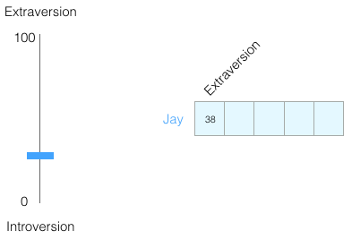
Suppose I scored 38 out of 100 for introversion / extraversion. This can be represented as follows:



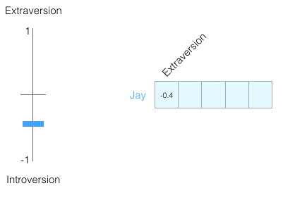
Or on a scale from −1 to +1:



How well do we recognize a person only by this assessment? Not really. People are complex creatures. Therefore we will add one more dimension: one more characteristic from the test.


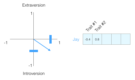
You can think of these two dimensions as a point on a graph or, even better, as a vector from the origin to this point. There are great tools for working with vectors that will come in handy very soon.

I do not show what personality traits we put on the chart so that you don’t become attached to specific traits, but immediately understand the vector representation of the personality of the person as a whole.

Now we can say that this vector partially reflects my personality. This is a useful description if you compare different people. Suppose I got hit by a red bus, and I need to replace me with a similar person. Which of the two people on the next chart is more like me?



When working with vectors, the similarity is usually calculated by the Otiai coefficient (geometric coefficient):


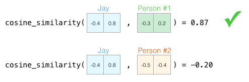
Man number 1 is more like me in character. Vectors in one direction (length is also important) give a larger Otiai coefficient

Again, two measurements are not enough to assess people. Decades of development of psychological science led to the creation of a test for five basic personality characteristics (with many additional ones). So let's use all five dimensions:



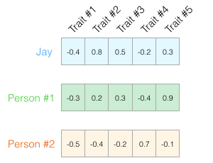
The problem with five dimensions is that it is no longer possible to draw neat arrows in 2D. This is a common problem in machine learning, where it is often necessary to work in multidimensional space. It is good that the geometric factor works with any number of measurements:


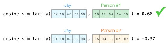
Geometric coefficient works for any number of measurements. In five dimensions, the result is much more accurate.

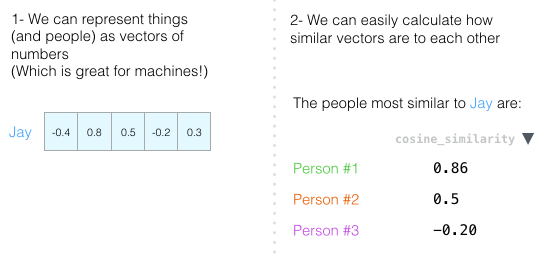
At the end of this chapter I want to repeat two main ideas:

1. People (and other objects) can be represented as numerical vectors (which is great for cars!).
   
2. We can easily calculate how similar the vectors are.

Word embedding

"The gift of words is the gift of deception and illusion." - Children of Dune

With this understanding, we turn to the vector representations of words obtained as a result of learning (they are also called embeddings) and look at their interesting properties.

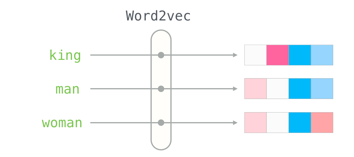
Here is an attachment for the word "king" (vector GloVe, trained on Wikipedia):

[ 0.50451 , 0.68607 , -0.59517 , -0.022801, 0.60046 , -0.13498 , -0.08813 , 0.47377 , -0.61798 , -0.31012 , -0.076666, 1.493 , -0.034189, -0.98173 , 0.68229 , 0.81722 , -0.51874 , -0.31503 , -0.55809 , 0.66421 , 0.1961 , -0.13495 , -0.11476 , -0.30344 , 0.41177 , -2.223 , -1.0756 , -1.0783 , -0.34354 , 0.33505 , 1.9927 , -0.04234 , -0.64319 , 0.71125 , 0.49159 , 0.16754 , 0.34344 , -0.25663 , -0.8523 , 0.1661 , 0.40102 , 1.1685 , -1.0137 , -0.21585 , -0.15155 , 0.78321 , -0.91241 , -1.6106 , -0.64426 , -0.51042 ]

We see a list of 50 numbers, but it’s difficult to say something about them. Let's visualize them to compare with other vectors. Put the numbers in one row:



Let's color the cells by their values ​​(red for close to 2, white for close to 0, blue for close to −2):



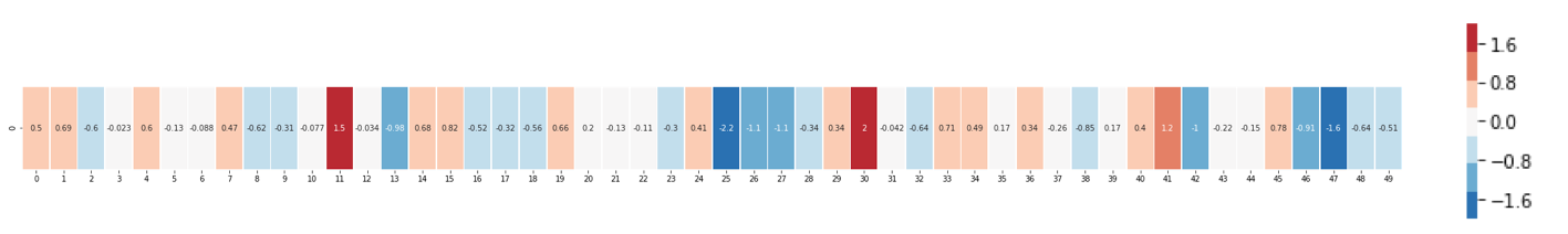
Now let's forget about the numbers, and only in colors we oppose the “king” with other words:



See that the "man" and "woman" are much closer to each other than to the "king"? It says something. Vector representations capture quite a lot of information / meaning / associations of these words.

Here is another list of examples (compare columns with similar colors):



You may notice a few things:

1. Through all the words goes one red column. That is, these words are similar in this particular dimension (and we do not know what is encoded in it).
   
2. You can see that “woman” and “girl” are in many ways similar. The same with "man" and "boy".
   
3. "Boy" and "girl" are also similar in some dimensions, but different from "woman" and "man." Perhaps this is coded vague idea of ​​youth? Probably.
   
4. Everything, except the last word, is a representation of people. I added an object (water) to show the differences between the categories. For example, you can see how the blue column goes down and stops in front of the “water” vector.
   
5. There are clear measurements, where the "king" and "queen" are similar to each other and differ from all others. Maybe there is encoded vague concept of royal power?

Analogies

“Words endure whatever burden we desire. All that is required for this is an agreement on tradition, according to which we build concepts. ” - God-emperor Dunes

Famous examples that show the incredible properties of investments - the concept of analogies. We can add and subtract word vectors to get interesting results. The most famous example is the formula “king is a man + woman”:


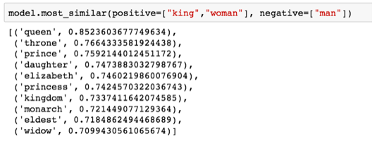
Using the Gensim library in python, we can add and subtract word vectors, and the library will find the words that are closest to the resulting vector. The image shows a list of the most similar words, each with a coefficient of geometric similarity

We visualize this analogy, as before:


The resulting vector from the “king – man + woman” calculation is not exactly equal to the “queen”, but this is the closest result of 400,000 word attachments in the data set

Having considered the attachments of words, let's explore how learning takes place. But before moving on to word2vec, you need to look at the conceptual ancestor of word embedding: the neural language model.

Language model

“The Prophet is not subject to the illusions of the past, present, or future. The fixedness of language forms determines such linear differences. The prophets hold the key to the tongue lock. For them, the physical image remains only a physical image and nothing more.

Their universe does not have the properties of a mechanical universe. A linear sequence of events is assumed by the observer. Cause and investigation? We are talking about something completely different. The Prophet expresses fateful words. You see a glimpse of an event that should happen “according to the logic of things”. But the prophet instantly releases the energy of infinite miraculous power. The universe is undergoing a spiritual shift. ” - God-emperor Dunes

One example of NLP (natural language processing) is the function of predicting the next word on the keyboard of a smartphone. Billions of people use it hundreds of times a day.



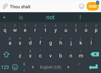
The prediction of the next word is a suitable task for the language model . She can take a list of words (say two words) and try to predict the following.

In the screenshot above, the model took these two green words ( thou shalt ) and returned a list of options (the highest probability for the word not ):



We can present the model as a black box:



But in practice, the model gives more than one word. It derives an estimate of the likelihood of virtually all known words (the “dictionary” of the model varies from a few thousand to over a million words). Then the keyboard application finds the words with the highest scores and shows them to the user.


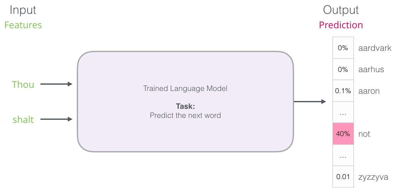
The neural model of the language gives the probability of all known words. We indicate probability in percent, but in the resulting vector, 40% will be represented as 0.4

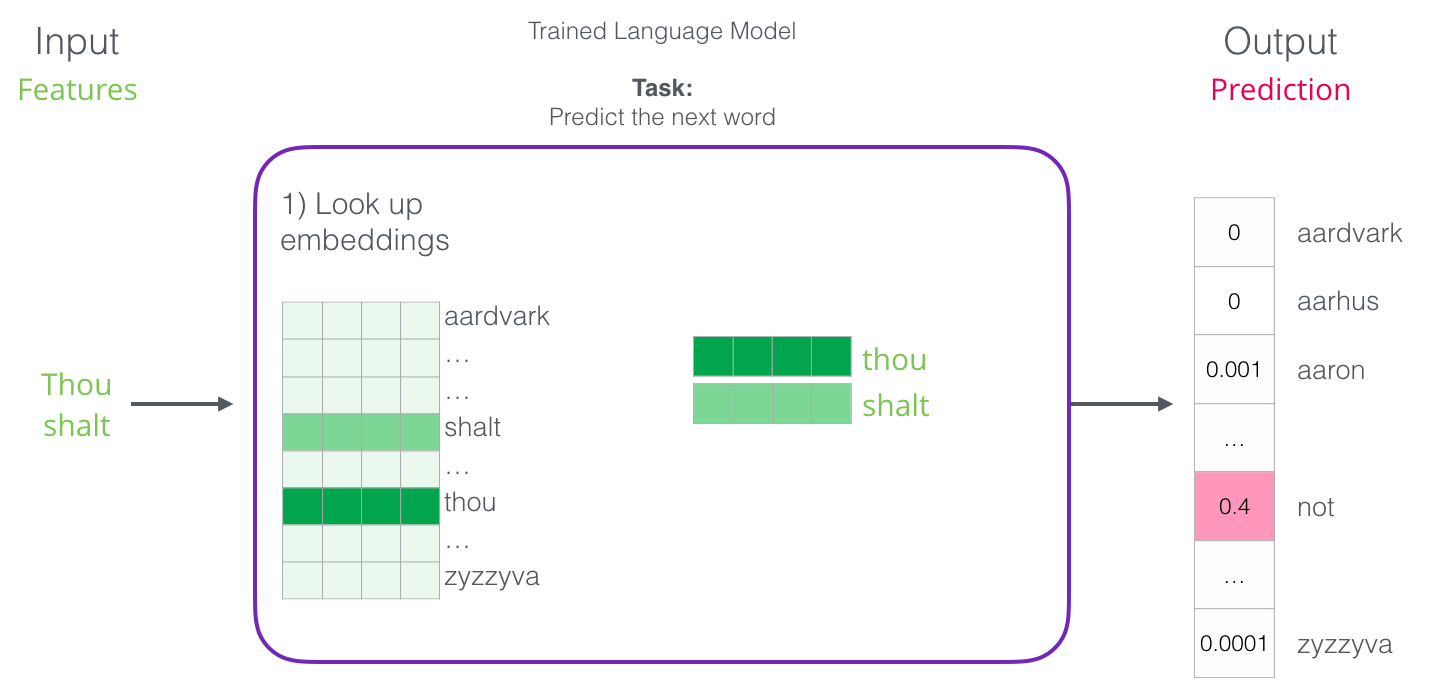
After training, the first neural models ( Bengio 2003 ) calculated the forecast in three stages:



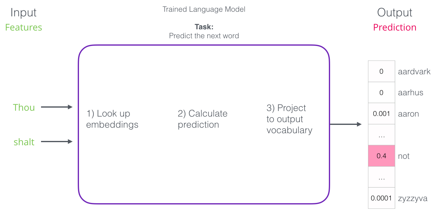
The first step for us is the most relevant, because we are discussing investments. As a result of the training, a matrix is ​​created with the attachments of all the words in our dictionary. To get the result, we simply look for the input word attachments and run the prediction:



Now let's look at the learning process and find out how this attachment matrix is ​​created.

Learning a language model

“The process cannot be understood by stopping it. Understanding should move with the process, merge with its flow and flow with it ”- Dune

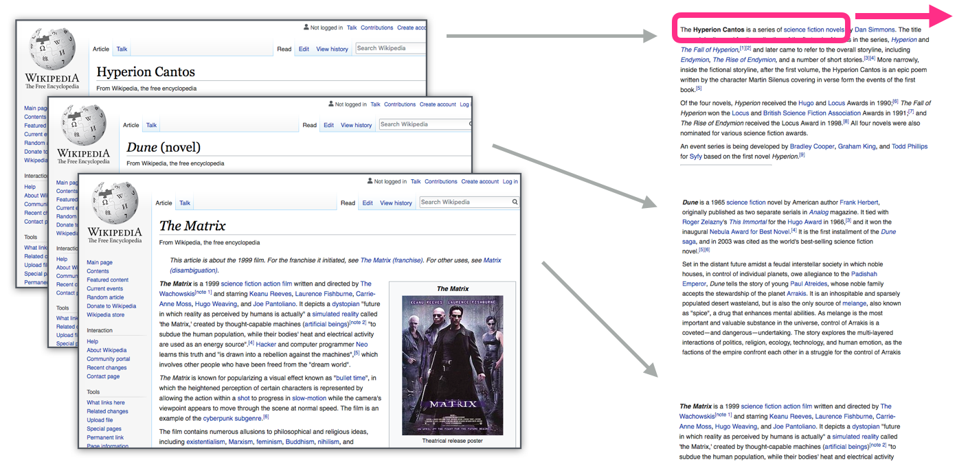
Language models have a huge advantage over most other machine learning models: they can be taught on texts that we have in abundance. Think of all the books, articles, Wikipedia materials and other forms of textual data that we have. Compare with other machine learning models that need manual labor and specially collected data.

“You must recognize the word from his company” - J. R. Furs

Attachments for words are calculated according to the surrounding words, which most often appear alongside. The mechanics are as follows:

1. We get a lot of text data (say, all Wikipedia articles)
   
2. Install a window (for example, of three words) that slides across the text.
   
3. A sliding window generates patterns to train our model.

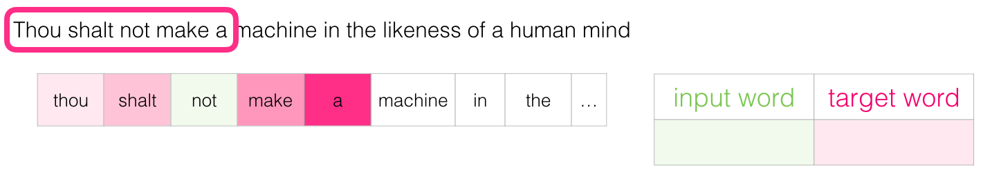
When this window slides through the text, we (actually) generate a data set, which we then use to train the model. To understand, let's see how a sliding window handles this phrase:

"Do not build a machine endowed with the likeness of the human mind" - Dune

When we start, the window is located on the first three words of the sentence:



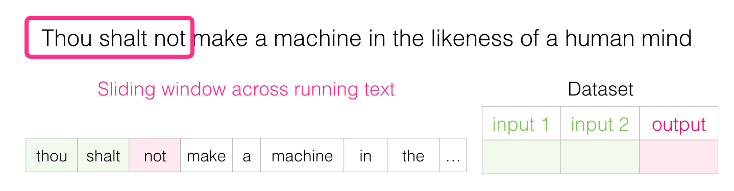
The first two words are taken as signs, and the third word is taken as a label:


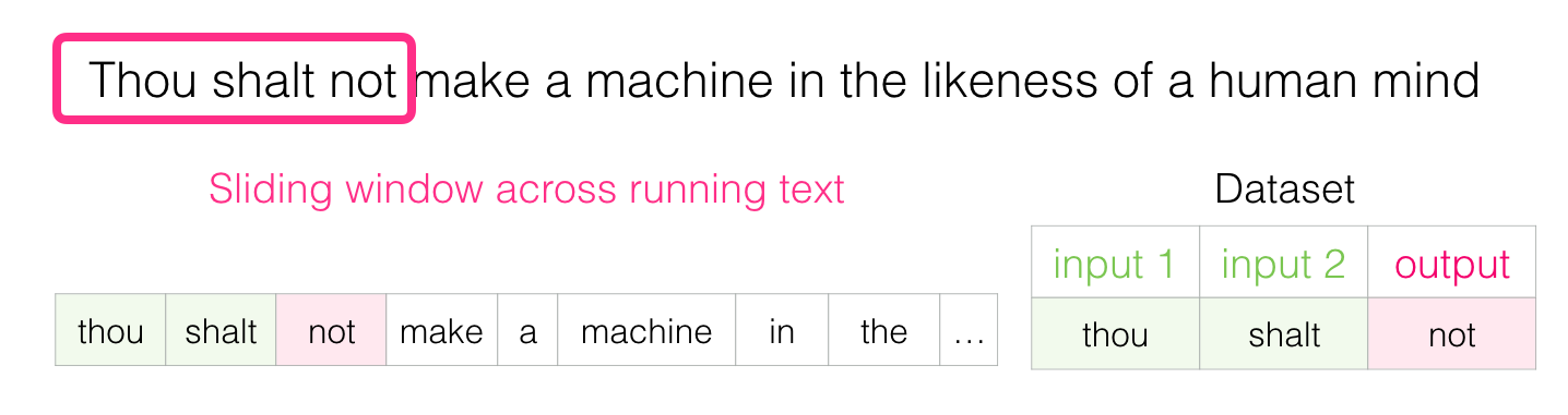
We generated the first sample in the data set, which can later be used to train a language model.

Then move the window to the next position and create the second sample:



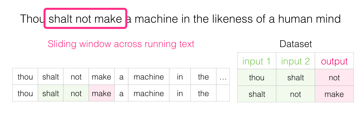
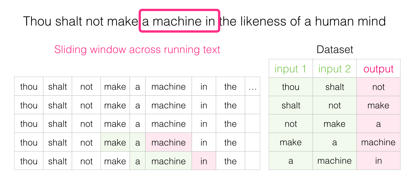
And pretty soon we have a larger set of data:



In practice, models are usually trained directly in the process of moving a sliding window. But logically, the “data set generation” phase is separated from the learning phase. In addition to neural network approaches, the N-gram method was often used to teach language models (see the third chapter of the book "Speech and Language Processing" ). To see the difference in the transition from N-grams to neural models in real products, here’s a post in 2015 on Swiftkey's blog , the developer of my favorite Android keyboard, which presents its neural language model and compares it with the previous N-gram model. I like this example because it shows how the algorithmic properties of an attachment can be described in a marketing language.

We look both ways

“The paradox is a sign that we must try to consider what lies behind it. If the paradox gives you concern, it means that you are striving for the absolute. Relativists view the paradox simply as an interesting, perhaps funny, sometimes scary thought, but a thought very instructive. ” God the emperor Dunes

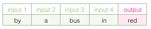
Taking into account all the above, fill in the gap:



As a context, there are five previous words (and the earlier mention of a “bus”). I am sure that most of you have guessed that there should be a “bus” here. But if I give you another word after the space, will it change your answer?



This completely changes the situation: now the missing word, most likely, is “red”. Obviously, there is informational value in words both before and after the space. It turns out that accounting in both directions (left and right) allows you to calculate higher-quality investments. Let's see how to adjust the training of the model in such a situation.

Skip-gram

"When an absolutely error-free choice is unknown, intelligence gets a chance to work with limited data in the arena, where mistakes are not only possible, but necessary." - Chapter Dunes

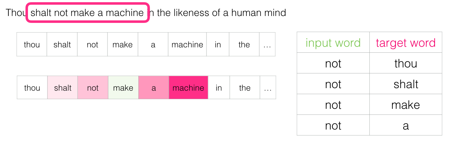
In addition to the two words before the target, you can take into account two more words after it.



Then the data set for learning the model will look like this:



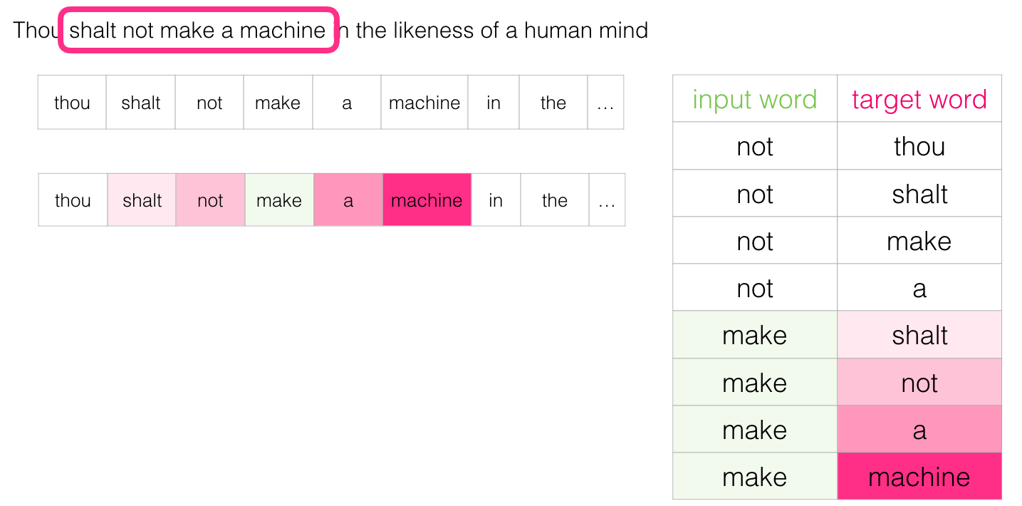
This is called the CBOW (Continuous Bag of Words) architecture and is described in one of the word2vec [pdf] documents . There is another architecture, which also show excellent results, but it works a little differently: it tries to guess the adjacent words using the current word. A sliding window looks like this:


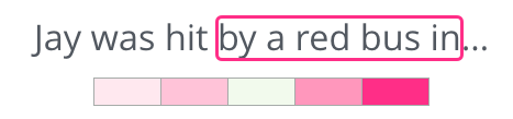
In the green slot is the input word, and each pink field represents a possible exit.

Pink rectangles have different shades, because this sliding window actually creates four separate patterns in our training data set:



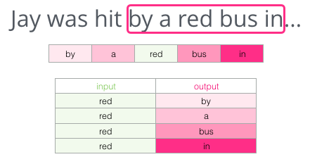
This method is called skip-gram architecture. You can visualize the sliding window as follows:



The following four samples are added to the training data set:



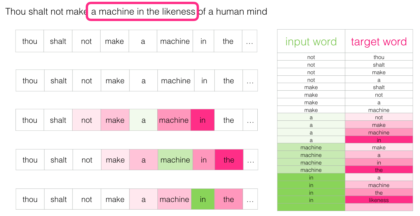
Then we move the window to the following position:



Which generates four more examples:



Soon we have much more samples:

Revision of the learning process

“Muad'Dib quickly learned because first of all he was taught how to learn. But the very first lesson was the assimilation of the belief that he can learn, and this is the basis of everything. It’s amazing how many people don’t believe in what they can learn and learn, and how many more people feel that it’s very difficult to learn. ” - Dune

Now that we have a set of skip-gram, we use it to teach a basic neural language model that predicts a neighboring word.



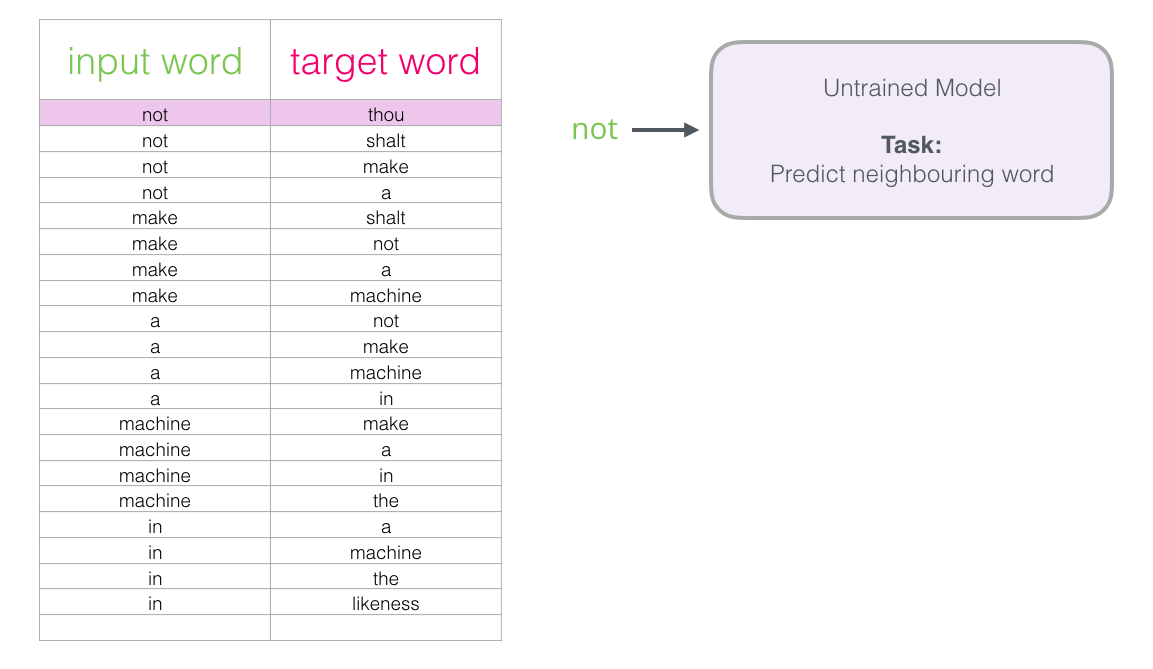
Let's start with the first sample in our data set. We take a sign and send it to the untrained model with a request to predict the adjacent word.



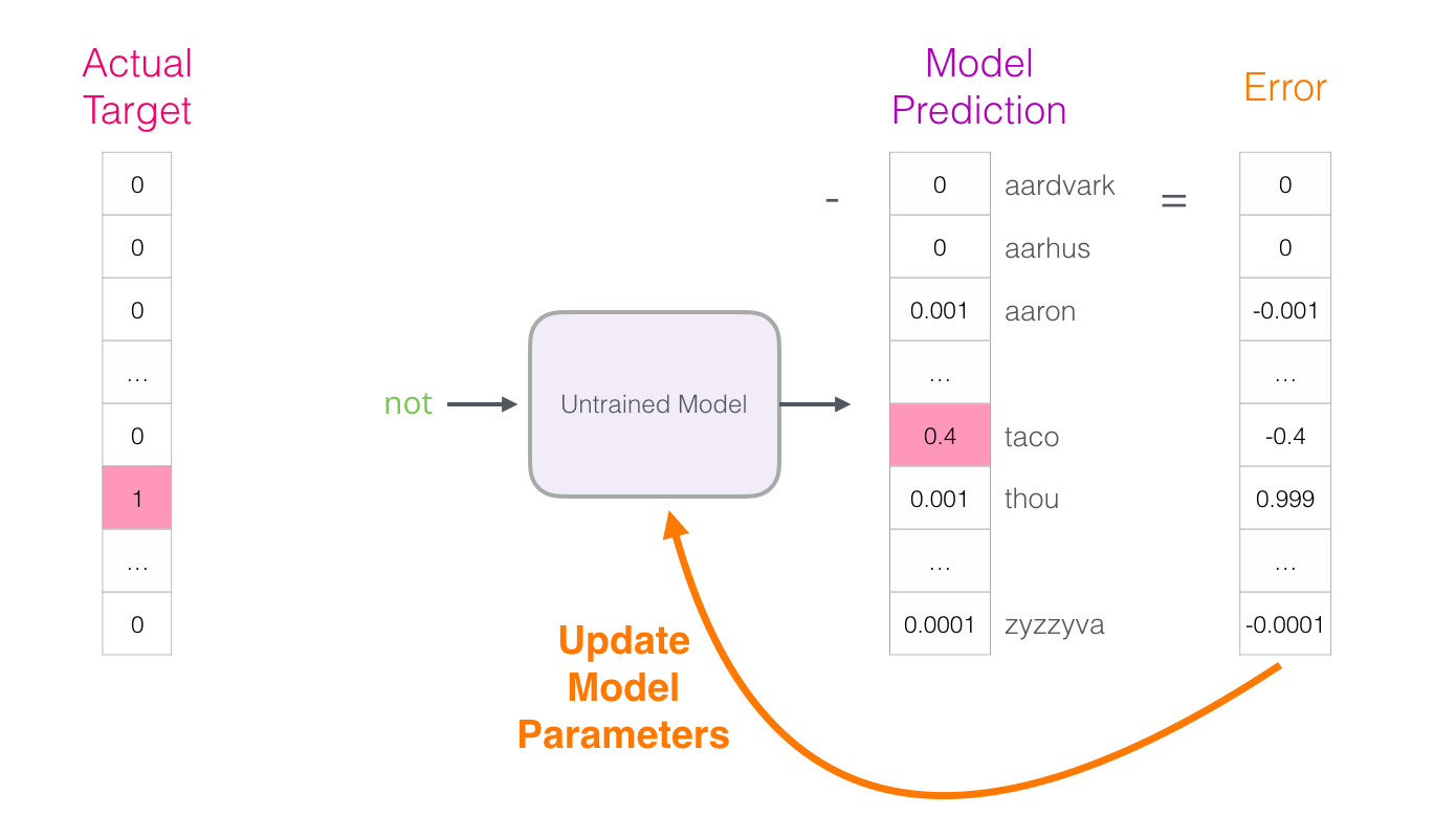
The model goes through three steps and displays the prediction vector (with probability for each word in the dictionary). Since the model is not trained, at this stage its prediction is probably incorrect. But it is nothing. We know what word it predicts - this is the resultant cell in the row that we currently use to train the model:


“Target vector” is the one in which the target word has a probability of 1, and all other words have a probability of 0

How wrong was the model? Subtract the forecast vector from the target and get the error vector:



This error vector can now be used to update the model, so the next time it is more likely to produce an exact result on the same input data.



Here the first stage of training is completed. We continue to do the same with the next sample in the dataset, and then with the next, until we look at all the samples. This is the end of the first era of learning. We repeat everything over and over again over several epochs, and as a result we get a trained model: from it we can extract the attachment matrix and use it in any applications.

Although we learned a lot, but to fully understand how word2vec really learns, a couple of key ideas are missing.

Negative selection

“Trying to understand Muad'Dib without understanding his mortal enemies, the Harkonnens, is the same thing as trying to understand the Truth without realizing what Lie is. This is an attempt to know the Light without knowing the Darkness. It's impossible". - Dune

Let us recall three stages, as the neural model calculates the prediction:



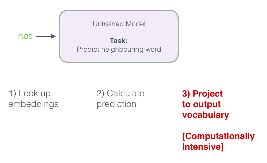
The third step is very expensive from the computational point of view, especially if you do it for each sample in the data set (tens of millions of times). It is necessary to somehow improve performance.

One way is to divide the goal into two stages:

1. Create high quality word attachments (without predicting the next word).
   
2. Use these high quality investments for language model training (for forecasting).

This article will focus on the first step. To increase performance, you can move away from predicting the next word ...



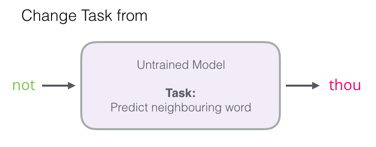
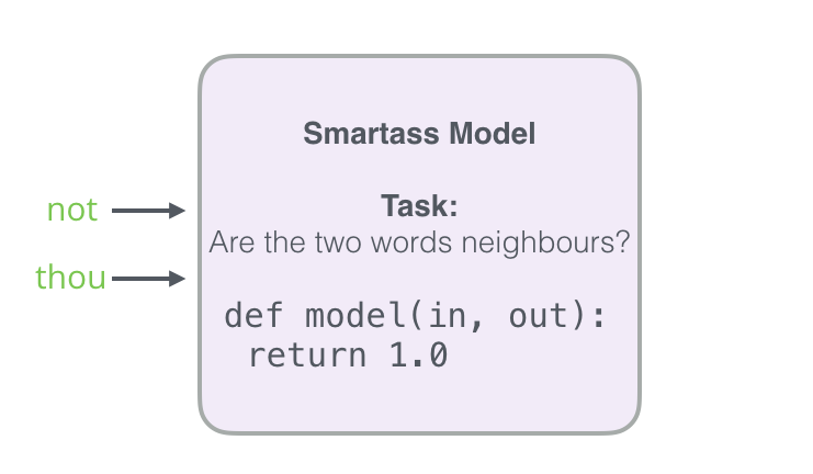
... and switch to a model that takes the input and output words and calculates the probability of their proximity (from 0 to 1).



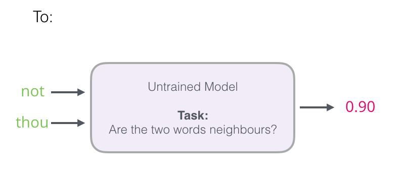
Such a simple transition replaces the neural network with a logistic regression model - thus, the calculations become much easier and faster.

At the same time, the structure of our dataset needs to be refined: the label is now a new column with values ​​of 0 or 1. In our table there is a unit everywhere, because we added neighbors there.



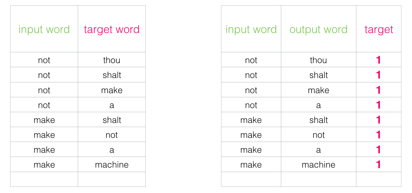
This model is calculated at an incredible speed: millions of samples in minutes. But you need to close one loophole. If all our examples are positive (goal: 1), then a tricky model can be formed that always returns 1, demonstrating 100% accuracy, but it does not learn anything and generates garbage attachments.



To solve this problem, you need to enter negative patterns into the data set — words that are not exactly neighbors. For them, the model is obliged to return 0. Now the model will have to work hard, but the calculations still go on at high speed.


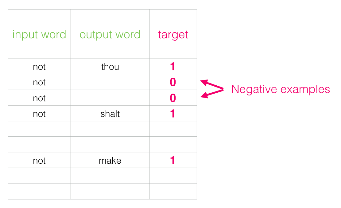
For each sample in the dataset add negative examples with label 0

But what to enter as output words? Choose words arbitrarily:



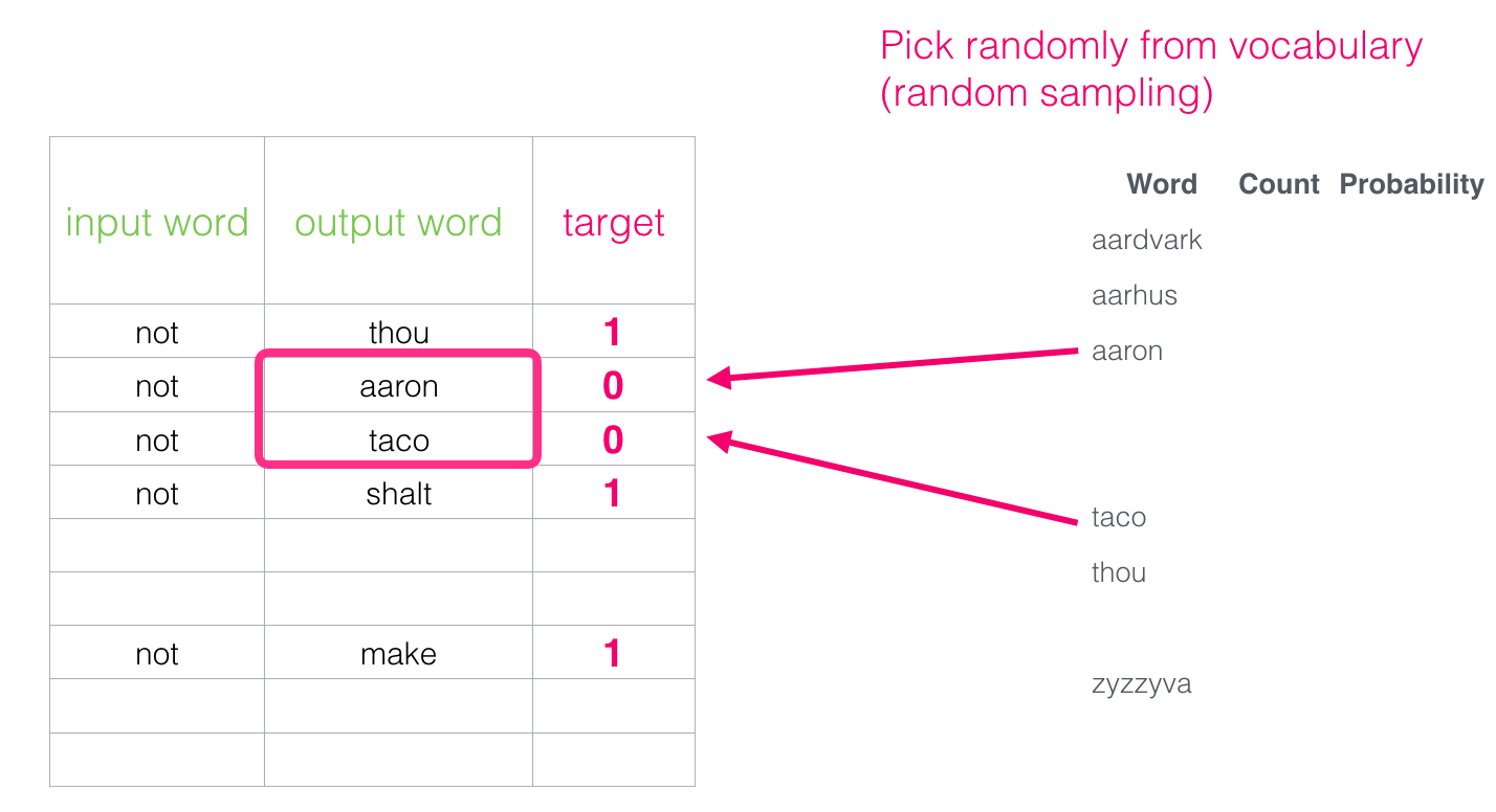
This idea was born under the influence of the noise-comparison estimation method [pdf]. We match the actual signal (positive examples of adjacent words) with noise (randomly selected words that are not neighbors). This provides an excellent trade-off between performance and statistical efficiency.

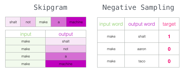
Skip-gram with negative sampling (SGNS)

We looked at two central concepts of word2vec: together they are called “skip-gram with negative sampling.”

Learning word2vec

“The machine cannot foresee every problem important to a living person. There is a big difference between discrete space and a continuous continuum. We live in one space, and machines exist in another. ” - God-emperor Dunes

Having analyzed the basic ideas of skip-gram and negative sampling, we can move on to a closer look at the word2vec learning process.

First, we pre-process the text on which we are training the model. We define the size of the dictionary (we will call it vocab_size ), say, 10,000 attachments and the parameters of words in the dictionary.

At the beginning of the training we create two matrices: Embedding and Context . Attachments for each word in our dictionary are stored in these matrices (therefore, vocab_size is one of their parameters). The second parameter is the dimension of the attachment (usually embedding_size set to 300, but earlier we considered an example with 50 dimensions).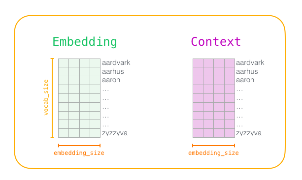



First, we initialize these matrices with random values. Then we begin the learning process. At each stage, we take one positive example and the associated negative ones. Here is our first group:



We now have four words: the input word not and the output / context words thou (actual neighbor), aaron and taco (negative examples). We start searching for their attachments in the Embedding matrices (for the input word) and Context (for context words), although both matrices contain attachments for all words from our dictionary.



Then we compute the scalar product of the input attachment with each of the context attachments. In each case, a number is obtained that indicates the similarity of the input data and contextual attachments.



Now we need a way to turn these estimates into some kind of probabilities: they should all be positive numbers between 0 and 1. This is a great problem for sigmoid logistic equations.



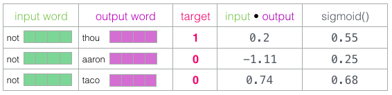
The result of the sigmoid calculation can be considered as the issuance of the model for these samples. As you can see, taco the highest score, while aaron still has the lowest score both before and after the sigmoid.

When the untrained model made a prediction and having a real target label for comparison, let's calculate how many errors in the model prediction. To do this, simply subtract the sigmoid estimate from the target labels.


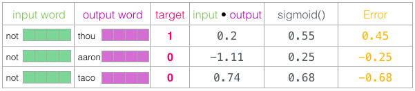
error = target - sigmoid_scores

Here comes the phase of "learning" from the term "machine learning". Now we can use this error estimate to adjust the not , thou , aaron and taco attachments so that the next calculation would result in a result closer to the target estimates.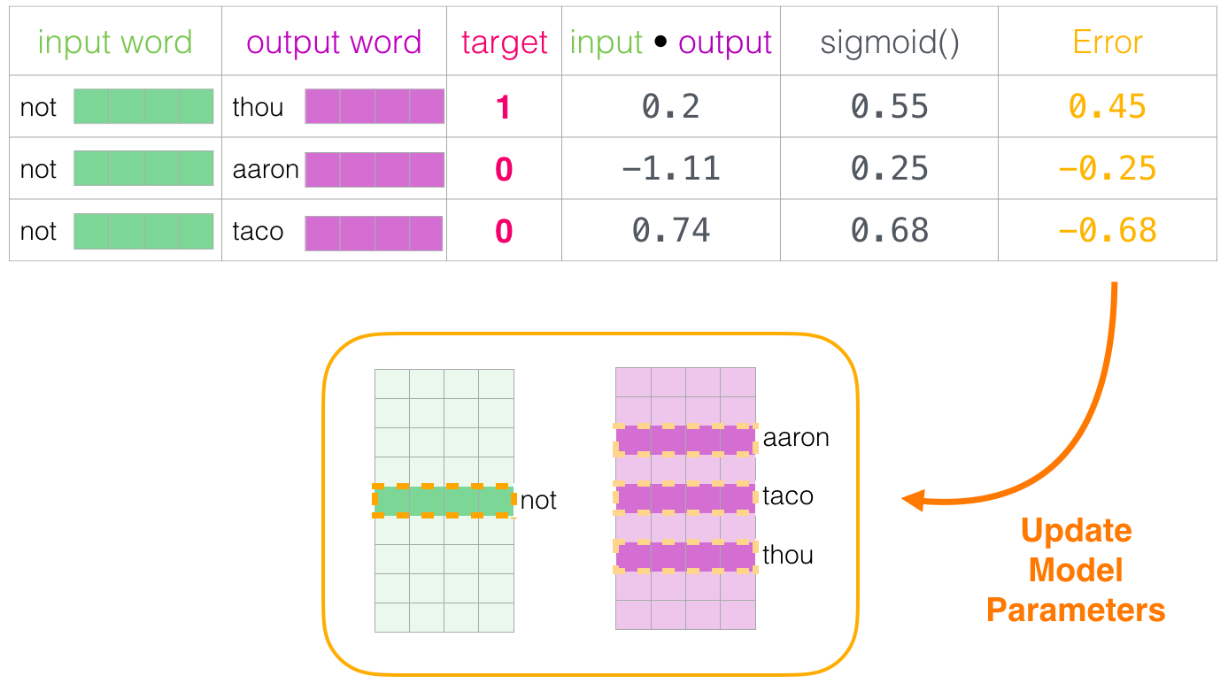



This completes one stage of training. We have slightly improved the embedding of several words ( not , thou , aaron and taco ). Now we go to the next stage (the next positive sample and the negative ones associated with it) and repeat the process.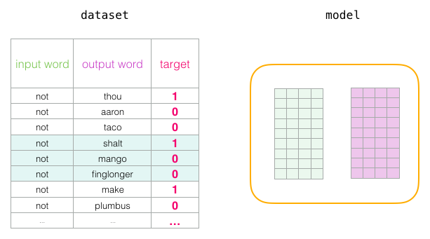



Attachments continue to improve as we cycle through the entire data set several times. You can then stop the process, put off the Context matrix, and use the trained Embeddings matrix for the next task.

Window size and number of negative samples

In the process of learning word2vec, two key hyperparameters are the window size and the number of negative samples.



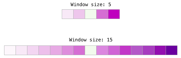
Different window sizes are suitable for different tasks. It is noticed that smaller windows (2−15) generate interchangeable attachments with similar indices (note that antonyms are often interchangeable when looking at the surrounding words: for example, the words “good” and “bad” are often mentioned in similar contexts). Larger window sizes (15–50 or even more) generate related investments with similar indices. In practice, you often have to provide annotations for the sake of useful semantic similarity in your task. In Gensim, the default window size is 5 (two words left and right, in addition to the input word itself).



The number of negative samples is another factor in the learning process. The original document recommends 5–20. It also states that 2–5 samples seem sufficient when you have a large enough data set. In Gensim, the default is 5 negative samples.

Conclusion

“If your behavior falls behind your measurements, then you are a living person, not an automaton” - God-emperor of Dune

I hope you now understand the attachments of words and the essence of the word2vec algorithm. I also hope that now you will understand the articles that mention the concept of “negative sampling gram” (SGNS), as in the aforementioned recommendation systems.

References and additional literature

• “Distributed representations of words and phrases and their composition” [pdf]
• « » [pdf]
• « » [pdf]
• « » — NLP. Word2vec .
• « » by — .
• Word2vec. « word2vec»
• ? :
  • word2vec Python Gensim
  • C ,
• « » , 2
• «»