Practical use of the D-Wave 2000Q: a steep learning curve for quantum computing

Rethinking the concept of a task is hard, but the result is worth it.

Author's note : I know that I incorrectly calculated the Bragg transference in both the classical and quantum cases; however, it is close enough to the truth in order to understand the difference between programming a classical and a quantum computer.

Time: somewhere in 2018. Location: the rotten canal in Slak.
')
"Do you know Python?"

Questions from John Timmer, scientific director of Ars Technica, can sometimes be taken by surprise. If in Slak it was possible to permeate the letters with caution, then my answer “Yes” would simply ooze it.

It turns out that D-Wave decided to give the world access to its quantum optimizer through an API. Ars invited him to try it out, but you had to know Python. I was ready for it.

I assumed that D-Wave would release some kind of fantastic API that could take my proprietary code that makes programmers cry, and turn it into quantum-optimized lines. Alas, when I got to the quantum optimizer, it turned out that it was not. I quickly found myself immersed in the documentation, trying to figure out what I really needed to do.

I think that the representative of D-Wave in public relations meant a person who knew enough to run ready-made examples. But I am stubborn. I needed to come up with three or four possible tasks that I wanted to check. I wanted to find out: can I master the process of solving these problems on a D-Wave computer? How easy is it to make a conceptual leap from classical programming to working with quantum annealing? Will any of my tasks even fit this machine?

Revealing a stunning conclusion right away, I will say that the answers were the following: maybe not quite “master”; complicated; not all tasks.

Selection of tasks for programming

Despite how you imagine me, you can call me a practicing programmer. In fact, anyone who is well versed in programming would have wrinkled (and, perhaps, would have committed a murder) upon seeing my Python code.

However, I can come up with tasks that require writing a program to solve them. I need, for example, something that calculates the electric field of a set of electrodes. Something that finds a state with minimal helium atom energy. Or something that counts the increase in light intensity at the start of the laser. These tasks interest me the most. And, having started this project, I had no idea whether the architecture of D-Wave can solve these problems.

I chose two problems that, in my opinion, could have worked: finding the members of the Mandelbrot set and calculating the potential contours of a set of electrodes. The advantage of these problems was that I could quickly solve them with classic code, and compare the answers. But I quickly ran into problems trying to figure out how to start solving these tasks on a D-Wave machine. It requires a serious shift in understanding the tasks, and my thinking works quite straightforwardly.

For example, one of the problems I encountered is that we are dealing with low-level binary numbers (despite the fact that they are expressed in the form of qubits, and not bits). This means that, in essence, there are no types in the program. Virtually all of my programming experience is in solving physical problems with floating point numeric types.

You have to think about the problem differently: the answer should be expressed as a binary number (ideally, true or false), and all physics (for example, all floating-point numbers) should be expressed through the union of qubits. Even if my life depended on it, I could not figure out how this can be done for any of my tasks. Immersed in teaching, I let this problem boil a little in my own juice.

Six months later, I finally came across a problem I was familiar with and which I could solve with the help of the D-Wave computer. The passage of light through the fiber Bragg grating can be expressed as a binary problem: did the photon come out of the filter, or not? All physics is contained in the compounds of qubits, and the answer is extracted from the energy of the solution.

Bragg grids

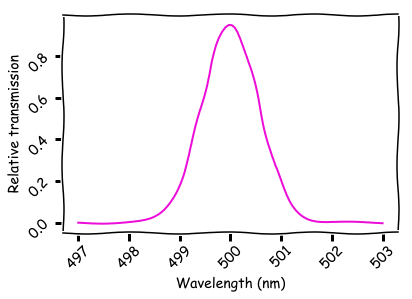
The one-dimensional Bragg grating is a multilayer material. Each gap between two layers reflects a small amount of light. The total penetration through the entire structure is determined by the distance between the gaps. In order for the light to pass through, it is necessary that the waves from different gaps add in phase. The aisle spectrum of an ideal Bragg grating with 50 layers and a reflectance of 0.1% is shown below.



The following code generates data for this graph:

ld = np.linspace(ld_center-3e-9, ld_center+3e-9, num_ld) k = 2*np.pi/ld T = np.ones(ld.shape) for j in range(num_layers): T = T*(1-A)*np.cos(j*k*layer_sep)**2 

Here we clearly calculate the relative contributions of each gap, expressed in optical power, which reach the next gap. Constructive and destructive interference is taken into account through a decrease or increase in the contribution of the gap, depending on how close the distance between the layers coincides with half the wavelength.

This hack is necessary, because the connection of qubits is expressed only in real, and not in complex numbers (physics is best expressed in terms of complex numbers containing the amplitude and phase of the light). Nevertheless, the output of the classic code looks approximately correct - a little worried about the lack of sidebands, which indicates that the model is incomplete, but so far it does not matter.

In the classic code, the model lacks consistency checks. I calculated the result, assuming exactly how the wave would propagate. Even if this assumption turns out to be wrong, the result of the calculation will be the same - although all equations are based on physics, it is impossible to guarantee in the code that they describe it correctly.

Go to quanta

In the D-Wave system it is necessary to create a chain of qubits, each of which represents the intensity of light on the gap. Each qubit is associated with neighbors, and the connection weight represents a passage from one gap to another, taking into account the distance between the interfaces. If the distance between the interfaces is half the wavelength, the light can resonate between the two interfaces and pass on. If the distance is equal to a quarter of the wavelength, destructive interference is triggered, and communication should be minimal.

Passing through one gap is indicated at 99.9%, so the connection between the zero and the first qubit is equal to

$$

$$P_ {0,1} = 0.999 cos ^ 2 (2 \ pi d / \ lambda)$$

Between the first and second:

$$

$$P_ {1,2} = P_ {0,1} 0.999 cos ^ 2 (4 \ pi d / \ lambda)$$

Between the second and third:

$$

$$P_ {2,3} = P_ {1,2} P_ {0,1} 0.999 cos ^ 2 (6 \ pi d / \ lambda)$$

In this formula, d denotes the physical distance between the layers, and λ is the wavelength. If d / λ = 0.5, then the cosine is equal to one, and we can hope for a perfect passage of light.

In the D-Wave system, this means that every two adjacent qubits should be connected as follows:

$$

$$P_ {i, j} = [0.999 cos ^ 2 (2i \ pi d / \ lambda)] ^ i$$

In this expression, the degree u takes into account the influence of previous qubits and simplifies the connection scheme.

Task implementation

Now, knowing how to connect qubits, we need to look at the physical connection of qubits to decide how to arrange this problem. This is called minor embedding.

We must give the computer a list of connections between the qubits with their weights. We must also specify deviations that indicate the importance of each qubit. In our case, all qubits are equally important, so they are set as -1 for all qubits (I took this number from the standard example). Deviations and connections must be associated with physical qubits and the connections between them. In the case of large tasks, the search for such a display may take a long time.

The code for generating connections and deviations is pretty simple.

  #qubit labels (q[j], q[j])       linear.update({(q[j], q[j]): -1}) #   #     if jk == -1: quad.update({(q[j], q[k]): (J_vals[j])**k}) #    else: quad.update({(q[j], q[k]): 0}) 

Fortunately, the D-Wave API will try to find a small implementation on its own. I found that it worked for a filter with 50 layers, but could not cope with 100 layers. This seems rather strange to me, since with 2000 qubits and a chain length of 1 (we don’t need to combine several physical qubits to create one logical one), the system should be able to implement larger problems. Looking back, I believe that the failure was due to the fact that I asked too many null links.

An alternative approach is simply not to define explicitly zero connections. This gives the algorithm the freedom to find more implementation options where qubits have no connections. I have not tried it, but this option seems to me to be the next logical step.

In any case, it is very easy to start the D-Wave machine:

 response = EmbeddingComposite(DWaveSampler()).sample_qubo(Q_auto, num_reads=num_runs) 

Learning to speak Qubit

The difference between my classic algorithm and the D-Wave solution is that the D-Wave computer does not directly return a clear result. It turns broken into many pieces. We get a list of energies, and the smallest of them should be the solution. For several runs (say, 1000) for each energy we get the number of times it appeared in the answer. And for each run we get the “answer”, the value of qubits. It was not immediately clear to me which of these values ​​can (and can) be interpreted as passing through a filter.

In the end, I decided that the minimum energy of the solution would best represent the answer, since this quantity in some sense represents the amount of energy stored in the filter. Therefore, a solution with more energy represents a greater permeability of the filter, as shown below. Turning this answer into a real passage of light is left as homework for those who understand this.



It is also possible to obtain a physical representation of the process by examining the values ​​of qubits at the solution with the lowest energy. Below you can see the bit solutions corresponding to the peak of the transmission curve (500 nm), 50% transmission (500.6 nm) and 5% transmission (501.4 nm).



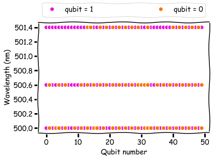
At the edge of the transmission peak, qubits tend to accumulate into groups of units. At the peak, the qubits alternate between 0 and 1. This last solution is a binary picture of how the light intensity varies in the Bragg grating. In other words, the D-Wave solution also represents physics directly, which cannot be said about my classic code.

This is the real power of quantum annealing. Yes, I can perfectly derive the curve of passing through the filter and from the classical calculations. But to get a picture of what is really happening inside, you need a more complex code. And in quantum annealing it goes completely free. In my opinion, this is very cool.

Another advantage of quantum annealing is that it guarantees the consistency of the solution as part of my choice of qubit link weights. This means that a quantum computer solution is likely to be more reliable than a solution derived from classical code.

Reasoning on quantum programming

The hardest thing in programming a D-Wave machine is that it requires a different way of thinking about tasks. I, for example, got used to minimization problems, when the curve coincides with the data. But I found it very difficult to change the way of thinking about the physical problem so as to start writing code to solve it. It does not help that most of the examples given by the company seem to me abstract and not adaptable to physical problems. But this situation will change when more and more users start publishing their code.

Also, difficulties may arise with the interpretation of the answer. Basically, I liked the simplicity of the API, and it's great to get additional ideas for free. In the near future, I could use D-Wave to solve real-world problems.