Reducing the sample size of experimental data without losing information

What is the problem of experimental data histograms

The basis for managing the quality of products of any industrial enterprise is the collection of experimental data and their subsequent processing.

Primary processing of experimental results includes comparing hypotheses about the law of data distribution, which describes the random value of the observed sample with the smallest error.
')
For this, the sample is presented in the form of a histogram consisting of $$$k$ columns built on intervals of length $$$d$ .

The identification of the form of distribution of measurement results also requires a number of problems, the solution efficiency of which is different for different distributions (for example, using the least squares method or calculating entropy estimates).

In addition, identification of the distribution is also needed because the scattering of all estimates (standard deviation, kurtosis, counter-process, etc.) also depends on the form of the distribution law.

The success of the identification of the form of the distribution of the experimental data depends on the sample size and, if it is small, the features of the distribution are masked by the randomness of the sample itself. In practice, to provide a large sample size, for example, more than 1000, is not possible for various reasons.

In such a situation, it is important to distribute the sample data in the best way at intervals, when for further analysis and calculations an interval series is necessary.

Therefore, for successful identification you need to solve the issue of assigning the number of intervals k

A. Khald in the book [1] convincingly argues that there is an optimal number of grouping intervals when the step envelope of the histogram built on these intervals is closest to the smooth distribution curve of the general population.

One of the practical signs of approaching the optimum can be the disappearance of dips in the histogram, and then closest to the optimum is considered the greatest k, at which the histogram still retains a smooth character.

Obviously, the type of histogram depends on the construction of the intervals of a random variable, however, even in the case of a uniform partition, there is still no satisfactory method of such a construction.

The splitting, which could be considered correct, leads to the fact that the error of approximation by a piecewise constant function of the supposedly continuous density distribution (histogram) will be minimal.

Difficulties due to the fact that the estimated density is unknown, so the number of intervals strongly affects the type of distribution of frequencies of the final sample.

With a fixed sample length, the enlargement of the partitioning intervals leads not only to clarifying the empirical probability of hitting them, but also to the inevitable loss of information (both in the general sense and in the sense of the probability density distribution curve), therefore, with further unjustified enlargement, the distribution being studied is too much smoothed .

Once having arisen, the task of optimal partitioning of the scope to the histogram does not disappear from the field of view of specialists, and until the only established opinion about its solution appears, the task will remain relevant.

The choice of criteria for assessing the quality of the histogram of experimental data

The Pearson's criterion, as is well known, requires dividing the sample into intervals — it is in them that the difference between the adopted model and the compared sample is evaluated.

$$$\ chi ^ {2} = \ sum_ {j = 1} ^ {m} \ frac {(E_ {j} -M_ {j}) ^ {2}} {M_ {j}}$

Where: $$$E_ {j}$ - experimental frequency values $$$(n_ {j})$ ; $$$M_ {j}$ - values ​​of frequencies in the same column; m is the number of histogram columns.

However, the application of this criterion in the case of intervals of constant length, usually used for constructing histograms, is inefficient. Therefore, in works on the effectiveness of the Pearson criterion, intervals are considered not with equal length, but with equal probability in accordance with the accepted model.

At the same time, however, the number of intervals of equal length and the number of intervals of equal probability differ by several times (except for an equiprobable distribution), which makes it possible to doubt the reliability of the results obtained in [2].

As a criterion of proximity, it is advisable to use the entropy coefficient, which is calculated as [3]:

$$$k_ {e} = \ frac {dn} {2 \ sigma} 10 ^ {\ beta}$

$$$\ beta = - \ frac {1} {n} \ sum_ {i = 1} ^ {m} {n_ {i} lg (n_ {i})}$

Where: $$$n_ {i}$ - the number of observations in the i-th interval $$$i = 0, ..., m$

Algorithm for assessing the quality of the histogram of experimental data using the entropy coefficient and the numpy.histogram module

The syntax for using the module is as follows [4]:

numpy.histogram (a, bins = m, range = None, normed = None, weights = None, density = None)

We will consider methods for finding the optimal number m of histogram partitioning intervals implemented in the numpy.histogram module:

• 'auto' - maximum ratings of 'sturges' and 'fd' , provides good performance;
• 'fd' (Freedman Diaconis Estimator) is a reliable (emission-resistant) estimator that takes into account data variability and size;
• 'doane' is an improved version of sturges assessment, which works more accurately with data sets with a distribution other than the normal one;
• 'scott' is a less reliable evaluator that takes into account the variability and size of the data;
• 'stone' - the evaluator is based on the cross-checking of the error square estimate, can be considered as a generalization of the Scott rule;
• 'rice' - the evaluator does not take into account the variability, but only the size of the data, often overestimates the number of required number of intervals;
• 'sturges' - a method (by default) that takes into account only the size of the data, is only optimal for Gaussian data and underestimates the number of intervals for large non-Gaussian data sets;
• 'sqrt' is the square root estimator of data size used by Excel and other programs for quick and simple calculations of the number of intervals.

To begin the description of the algorithm, we adapt the numpy.histogram () module to calculate the entropy coefficient and the entropy error:

from numpy import* def diagram(a,m,n): z=histogram(a, bins=m) if type(m) is str:#       m=len(z[0]) y=z[0] d=z[1][1]-z[1][0]#   h=0.5*d*n*10**(-sum([w*log10(w) for w in y if w!=0])/n)#  ke=h/std (a)#    (1). return ke,h 

Now consider the main stages of the algorithm:

1) We form a control sample (hereinafter referred to as the “large sample”) that meets the requirements for experimental data processing error . From a large sample by removing all the odd members we form a smaller sample (hereinafter referred to as the “small sample”);

2) For all evaluators 'auto', 'fd', 'doane', 'scott', 'stone', 'rice', 'sturges', 'sqrt', we calculate the entropy coefficient ke1 and the error h1 for a large sample and the entropy coefficient ke2 and the error h2 on a small sample, as well as the absolute value of the difference - abs (ke1-ke2);

3) Controlling the numerical values ​​of the evaluators at the level of at least four intervals, we choose an evaluator that provides the minimum value of the absolute difference - abs (ke1-ke2).

4) For the final decision, the appraiser is selected on one distribution histogram for a large and small sample with an appraiser providing the minimum abs value (ke1-ke2), and the second one with an appraiser providing the maximum abs value (ke1-ke2). The appearance of additional jumps in a small sample on the second histogram confirms the correctness of the choice of the evaluator at the first.

Consider the work of the proposed algorithm for sampling data from the publication [2]. The data were obtained by random selection of 80 blanks from 500, followed by measuring their mass. The stock must have a mass within the following limits: $$$m = 17 _ {- 0.4} ^ {+ 0.6}$ kg The optimal parameters of the histogram will be determined using the following listing:


We get:

The standard deviation for the sample (n = 80): 0.24
Mathematical expectation for sample (n = 80): 17.158
The standard deviation for the sample (n = 40): 0.202
The mathematical expectation of the sample (n = 40): 17.138
ke1 = 1.95, h1 = 0.467, ke2 = 1.917, h2 = 0.387, dke = 0.033, m = auto
ke1 = 1.918, h1 = 0.46, ke2 = 1.91, h2 = 0.386, dke = 0.008, m = fd
ke1 = 1.831, h1 = 0.439, ke2 = 1.917, h2 = 0.387, dke = 0.086, m = doane
ke1 = 1.918, h1 = 0.46, ke2 = 1.91, h2 = 0.386, dke = 0.008, m = scott
ke1 = 1.898, h1 = 0.455, ke2 = 1.934, h2 = 0.39, dke = 0.036, m = stone
ke1 = 1.831, h1 = 0.439, ke2 = 1.917, h2 = 0.387, dke = 0.086, m = rice
ke1 = 1.95, h1 = 0.467, ke2 = 1.917, h2 = 0.387, dke = 0.033, m = sturges
ke1 = 1.831, h1 = 0.439, ke2 = 1.917, h2 = 0.387, dke = 0.086, m = sqrt



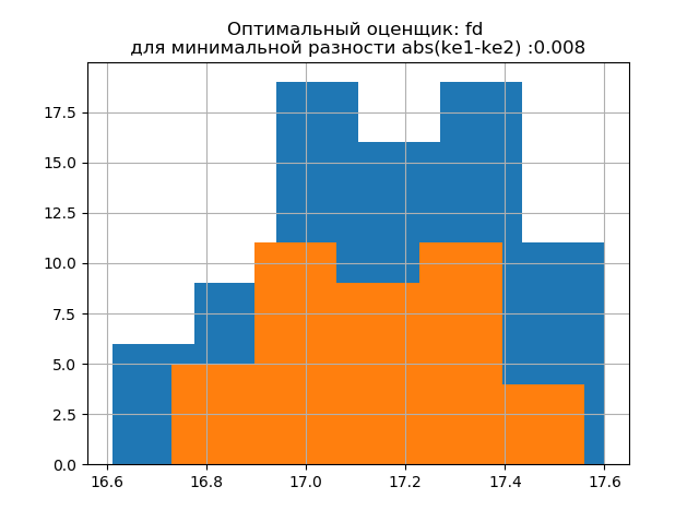
The form of distribution of a large sample is similar to the form of distribution of a small sample. As follows from the writing, 'fd' is a reliable (emission resistant) estimator that takes into account the variability and size of the data. In this case, the entropy error of a small sample even decreases slightly: h1 = 0.46, h2 = 0.386 with a slight decrease in the entropy coefficient from k1 = 1.918 to k2 = 1.91.



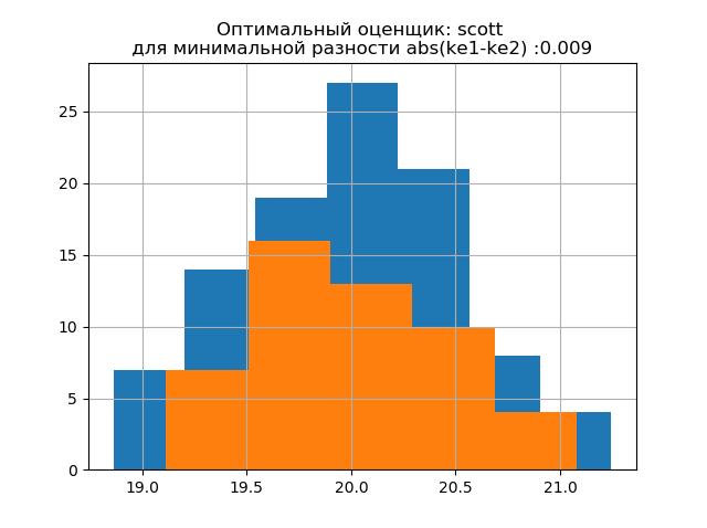
The distribution patterns of large and small samples vary. As follows from the description, 'doane' is an improved version of the 'sturges' rating, which works better with data sets with a distribution other than the normal one. In both samples, the entropy coefficient is close to two, and the distribution is close to normal. The appearance of additional jumps in a small sample on this histogram, compared with the previous one, additionally indicates the correct choice of the 'fd' evaluator.

We generate new two samples for the normal distribution with the parameters mu = 20, sigma = 0.5 and size = 100 using the relation:

 a= list([round(random.normal(20,0.5),3) for x in arange(0,100,1)]) 

The developed method is applicable to the obtained sample using the following program:



We get:
The standard deviation for the sample (n = 100): 0.524
Mathematical expectation for sample (n = 100): 19.992
The standard deviation for the sample (n = 50): 0.462
Expectation Sample (n = 50): 20.002
ke1 = 1.979, h1 = 1.037, ke2 = 2.004, h2 = 0.926, dke = 0.025, m = auto
ke1 = 1.979, h1 = 1.037, ke2 = 1.915, h2 = 0.885, dke = 0.064, m = fd
ke1 = 1.979, h1 = 1.037, ke2 = 1.804, h2 = 0.834, dke = 0.175, m = doane
ke1 = 1.943, h1 = 1.018, ke2 = 1.934, h2 = 0.894, dke = 0.009, m = scott
ke1 = 1.943, h1 = 1.018, ke2 = 1.804, h2 = 0.834, dke = 0.139, m = stone
ke1 = 1.946, h1 = 1.02, ke2 = 1.804, h2 = 0.834, dke = 0.142, m = rice
ke1 = 1.979, h1 = 1.037, ke2 = 2.004, h2 = 0.926, dke = 0.025, m = sturges
ke1 = 1.946, h1 = 1.02, ke2 = 1.804, h2 = 0.834, dke = 0.142, m = sqrt



The form of distribution of a large sample is similar to the form of distribution of a small sample. As follows from the description, 'scott' is a less reliable estimator, taking into account the variability and size of data. In this case, the entropy error of a small sample even decreases slightly: h1 = 1,018 and h2 = 0,894 with a slight decrease in the entropy coefficient from k1 = 1,943 to k2 = 1,934. . It should be noted that for the new sample we obtained the same tendency of changing the parameters as in the previous example.



The distribution patterns of large and small samples vary. As follows from the description, 'doane' is an improved version of the 'sturges' rating , which more accurately works with data sets with a distribution other than the normal one. In both samples, the distribution is normal. The appearance of additional jumps in the small sample on this histogram compared to the previous one additionally indicates the correct choice of the 'scott' evaluator.

The use of smoothing for comparative analysis of histograms

Smoothing histograms built on a large and small sample allows us to more accurately determine their identity in terms of preserving the information contained in a sample of a larger volume. Imagine the last two histograms as smoothing functions:




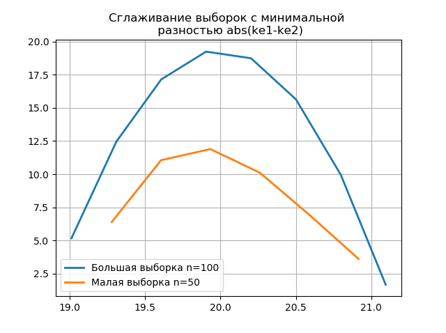
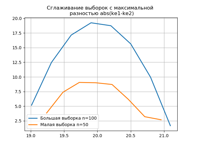
The appearance of additional jumps in a small sample on the graph of the smoothed histogram compared with the previous one additionally indicates the correct choice of the 'scott' evaluator.

findings

The calculations given in the article in the range of small samples common in the production confirmed the efficiency of using the entropy coefficient as a criterion for preserving the information content of the sample while reducing its volume . The technique of applying the latest version of the numpy.histogram module with built-in evaluators - 'auto', 'fd', 'doane', 'scott', 'stone', 'rice', 'sturges', 'sqrt', which is enough for optimization analysis of experimental data on interval estimates.

References:

1. Hald A. Mathematical statistics with technical applications. - Moscow: Izd-voinoostr. lit., 1956
2. Kalmykov V.V., Antonyuk F.I., Zenkin N.V.
Determination of the optimal number of grouping classes of experimental data with interval estimates // South Siberian Scientific Bulletin.— 2014.— No. 3. —C. 56–58.
3. Novitsky P.V. The concept of the entropy value of the error // Measuring equipment. —1966.— № 7. —S. 11-14.
4. numpy.histogram - NumPy v1.16 Manual