Dynamic remarketing (dynrem) in myTarget is a targeted advertising technology that uses information about user actions on websites and mobile applications of advertisers. For example, in an online store, a user viewed product pages or added them to the cart, and myTarget uses these events to display advertisements for exactly those goods and services to which a person has previously shown interest. Today I will talk more about the mechanism for generating non-personal, that is, item2item-recommendations, which allow to diversify and supplement the advertising issue.

The clients for dynrem myTarget are mainly online stores, which may have one or several lists of goods. When building recommendations, the pair “store - list of goods” must be taken into account as a separate unit. But for simplicity, we will continue to use just the “store” If we talk about the dimension of the problem at the entrance, then recommendations need to be built for about a thousand stores, and the quantity of goods can vary from a few thousand to millions.

The recommendation system for dynrem must meet the following requirements:
')

1. The banner contains products that maximize its CTR.
2. Recommendations are built in offline mode for a specified time.
3. The system architecture must be flexible, scalable, resilient, and operate in a cold start.

Note that from the requirement of building recommendations for a fixed time and the described initial conditions (we will optimistically assume that the number of stores is increasing) naturally arises the requirement of economical use of machine resources.

Section 2 contains the theoretical basis for building recommender systems, sections 3 and 4 deal with the practical side of the issue, and section 5 summarizes.

Basic concepts

Consider the task of building a recommender system for one store and list the main mathematical approaches.

Singular Value Decomposition (SVD)

A popular approach to building recommender systems is the singular value decomposition (SVD) approach. Matrix ratings $$$R = (r_ {ui})$ represent as a product of two matrices $$$P$ and $$$Q$ so that $$$R \ approx P Q ^ T$ , then user rating rating $$$u$ for goods $$$i$ represented as $$$\ hat {r} _ {ui} = <p_u, q_i>$ [1], where the elements of the scalar product are dimension vectors $$$k$ (the main parameter of the model). This formula serves as the basis for other SVD models. Task of finding $$$P$ and $$$Q$ comes down to optimizing the functional:

(2.1)

$$

$$J (P, Q) = \ sum _ {(u, i)} \ mathcal {L} (r_ {ui}, \ hat {r} _ {ui}) + \ Lambda (P, Q) \ rightarrow \ min_ {P, Q},$$

Where $$$L$ - error function (for example, RMSE as in a Netflix contest), $$$Λ$ - regularization, and summation goes in pairs, for which the rating is known. We rewrite expression (2.1) explicitly:

(2.2)

$$

$$J (P, Q) = \ sum _ {(u, i)} (r_ {ui} - <p_u, q_i>) ^ 2 + \ lambda_1 || p_u || ^ 2 + \ lambda_2 || q_i || ^ 2 \ rightarrow \ min_ {P, Q},$$

Here $$$λ1$ , $$$λ2$ - L2 regularization coefficients for user views $$$p_ {u}$ and product $$$q_ {i}$ respectively. The basic model for the Netflix competition was:

(2.3)

$$

$$\ hat {r} _ {ui} = \ mu + b_u + b_i + <p_u, q_i>,$$

(2.4)

$$

$$J (P, Q) = \ sum _ {(u, i)} (r_ {ui} - \ mu - b_u - b_i - <p_u, q_i>) ^ 2 + \ lambda_1 || p_u || ^ 2 + \ lambda_2 || q_i || ^ 2 + \ lambda_3 b_u ^ 2 + \ lambda_4 b_i ^ 2 \ rightarrow \ min_ {P, Q},$$

Where $$$µ$ , $$$b_ {u}$ and $$$b_ {i}$ - Offsets for rating, user and product, respectively. Model (2.3) - (2.4) can be improved by adding an implicit user preference to it. On the example of a Netflix competition, the explicit response is the score given by the user to the film “at our request”, and the implicit response is other information about the “user interaction with the product” (watching the film, its description, reviews on it; i.e. an implicit response does not direct information about the rating of the film, but it indicates interest). Consideration of the implicit response is implemented in the SVD ++ model:

(2.5)

$$

$$\ hat {r} _ {ui} = \ mu + b_u + b_i + <p_u + \ frac {1} {\ sqrt {\ sigma_u}} \ sum_ {j \ in S (u)} y_j, \, \ , q_i>,$$

Where $$$S (u)$ - a set of objects with which the user implicitly interacted, $$$σ_ {u} = | S (u) |, y_ {j}$ - representation of dimension $$$k$ for an object of $$$S (u)$ .

Factorization Machines (FM)

As seen in the examples with different SVD models, one model differs from another in the set of terms included in the evaluation formula. In this case, the expansion of the model each time represents a new task. We want such changes (for example, adding a new kind of implicit response, taking into account time parameters) to be easily implemented without changing the model implementation code. Models (2.1) - (2.5) can be represented in a convenient universal form using the following parameterization. We represent the user and product in the form of a set of signs:

(2.6)

$$

$$\ overline {x} ^ U = (x_1 ^ U, x_2 ^ U, \ dots, x_l ^ U) \ in \ mathbb {R} ^ l,$$

(2.7)

$$

$$\ overline {x} ^ I = (x_1 ^ I, x_2 ^ I, \ dots, x_m ^ I) \ in \ mathbb {R} ^ m.$$

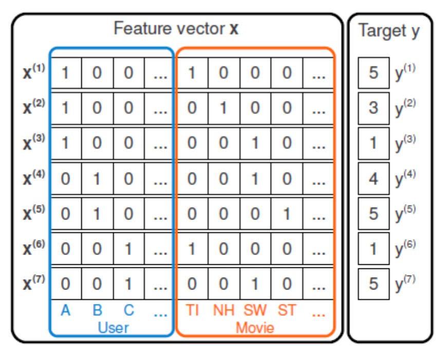
Fig. 1: An example of a feature matrix in the case of CF.

For example, in the case of collaborative filtering (CF), when only data on the interaction of users and products are used, feature vectors are in the form of a one-hot code (Fig. 1). We introduce a vector $$$\ overline {x} = (\ overline {x} ^ U, \ overline {x} ^ I)$ then the recommendation task is reduced to regression tasks with the target variable $$$r_ {ui}$ :

1. Linear model:
   (2.8)
   

   $$

   $$h_ {lin} (\ overline {x}) = w_0 + \ sum_ {j = 1} ^ {l + m} w_jx_j$$
2. Poly2:
   (2.9)
   

   $$

   $$h_ {poly2} (\ overline {x}) = w_0 + \ sum_ {j = 1} ^ {l + m} w_jx_j + \ sum_ {i = 1} ^ {l + m} \ sum_ {j = i + 1 } ^ {l + m} w_ {ij} x_i x_j$$
3. FM:
   (2.10)
   

   $$

   $$h_ {FM} (\ overline {x}) = w_0 + \ sum_ {j = 1} ^ {l + m} w_jx_j + \ sum_ {i = 1} ^ {l + m} \ sum_ {j = i + 1 } ^ {l + m} x_i x_j <\ overline {v} _i, \ overline {v} _j>$$

Where $$$w_ {j}$ - model parameters, $$$v_ {i}$ - dimension vectors $$$k$ representing the attribute $$$i$ in latent space, $$$l$ and $$$m$ - the number of signs of the user and product, respectively. In addition to one-hot-codes, content attributes (Content-based, CB) (Fig. 2), for example, vectorized descriptions of products and user profiles, can act as attributes.


Fig. 2: Example of an extended feature matrix.

The FM model introduced in [2] is a generalization for (2.1) - (2.5), (2.8), (2.10). The essence of FM is that it takes into account the pairwise interaction of features using the scalar product $$$<\ overline {v} _i, \ overline {v} _j>$ rather than using the parameter $$$w_ {ij}$ . The advantage of FM relative to Poly2 is to significantly reduce the number of parameters: for vectors $$$v_ {i}$ we will need $$$(l + m) · k$ parameters, and for $$$w_ {ij}$ would need $$$l · m$ parameters. With $$$l$ and $$$m$ large orders, the first approach uses significantly fewer parameters.

Note: if there is no specific pair in the training set $$$(i, j)$ , then the corresponding term with $$$w_ {ij}$ in Poly2, it does not affect the training of the model, and the rating of the rating is formed only along the linear part. However, approach (2.10) allows you to establish links through other signs. In other words, the data on one interaction helps to estimate the parameters of features not included in this example.

On the basis of FM, a so-called hybrid model is implemented, in which CB-signs are added to CF signs. It allows you to solve the problem of cold start, and also takes into account user preferences and allows you to make personal recommendations.

Lightfm

In the popular implementation of FM , emphasis is placed on the separation between user and product attributes. The parameters of the model are matrices. $$$E ^ u$ and $$$E ^ i$ Submission of custom and product features:

(2.11)

$$

$$E ^ U = \ begin {pmatrix} \ overline {e} _1 ^ U \\ \ vdots \\ \ overline {e} _l ^ U \ end {pmatrix}, \, \, E ^ I = \ begin {pmatrix } \ overline {e} _1 ^ I \\ \ vdots \\ \ overline {e} _m ^ I \ end {pmatrix}, \ overline {e} _i ^ U \ in \ mathbb {R} ^ k, \ overline { e} _i ^ I \ in \ mathbb {R} ^ k$$

as well as offsets $$$\ overline {b} ^ U, \ overline {b} ^ I \ in \ mathbb {R} ^ k$ . Using user and product views:

(2.12)

$$

$$\ overline {p} ^ U = \ overline {x} ^ U \ cdot E ^ U = \ sum_ {j = 1} ^ l x_j ^ U \ cdot \ overline {e} _j ^ U,$$

(2.13)

$$

$$\ overline {q} ^ I = \ overline {x} ^ I \ cdot E ^ I = \ sum_ {j = 1} ^ m x_j ^ I \ cdot \ overline {e} _j ^ I,$$

get pair rating $$$(u, i)$ :

(2.14)

$$

$$\ hat {r} _ {ui} = <\ overline {p} ^ U, \ overline {q} ^ I> + <\ overline {x} ^ U, \ overline {b} ^ U> + <\ overline {x} ^ I, \ overline {b} ^ I>.$$

Loss functions

In our case, it is necessary to arrange the goods for a specific user so that the more relevant product has a higher rating than the less relevant one. LightFM implements several loss functions:

1. Logistic is an implementation that requires a negative, which is not explicitly represented in most tasks.
2. BPR [3] is to maximize the difference in ratings between positive and negative examples for a particular user. Negative is obtained by bootstrap sampling. The quality functionality used in the algorithm is similar to the ROC-AUC.
3. WARP [4] differs from BPR by sampling negative examples and the loss function, which is also ranking, but also optimizes the top recommendations for the user.

Practical implementation

To build recommendations for a specified time, a parallel implementation on Spark is used. For each store, an independent task is started, the execution of which is controlled by luigi.

Data preprocessing

Data preprocessing is performed by automatically scaled Spark SQL tools. The attributes selected for the final model are text descriptions of goods and catalogs with standard transformations.

What helped us in dealing with Spark:

1. Partitioning of the prepared data (matrix of interactions of users and products, signs for them) in the shops. This allows you to save time reading data from HDFS at the training stage. Otherwise, each task has to read the data into the Spark memory and filter it by store ID.
2. Saving / retrieving data to / from Spark is done in parts. This is due to the fact that in the process of any of these actions, the data is loaded into the memory of the JVM. Why not just increase the memory for the JVM? First, then the memory available for learning the model is reduced, and secondly, it is not necessary to store anything in the JVM, it acts in this case as a temporary storage.

Model training

The model for each store is trained in its Spark-container, so that you can simultaneously run an arbitrary number of tasks for stores, limited only by cluster resources.

In LightFM, there are no early stop mechanisms, therefore, we spend extra resources on additional learning iterations when there is no target metric gain. We chose AUC as a metric, the relationship of which with CTR is confirmed experimentally.

Denote:

$$$S$ - all known interactions between users and products, that is, pairs $$$(u, i)$ ,
$$$I$ - the set of all goods $$$i$ ,
$$$U$ - many all users $$$u$ .
For a specific user $$$u$ also introduce $$$I_ {u} = {i ∈ I: (u, i) ∈ S}$ - many products with which the user interacts. AUC can be calculated as follows [ref]:

(3.1)

$$

$$AUC (u) = \ frac {1} {| \ mathcal {I} _u || \ mathcal {I} \ setminus \ mathcal {I} _u |} \ sum_ {i \ in \ mathcal {I} _u} \ sum_ {j \ in \ mathcal {I} \ setminus \ mathcal {I} _u} \ delta (\ hat {r} _ {ui}> \ hat {r} _ {uj}),$$

(3.2)

$$

$$AUC = \ frac {1} {| \ mathcal {U} |} \ sum_ {u \ in \ mathcal {U}} AUC (u).$$

In formula (3.1) we need to calculate the rating for all possible pairs. $$$(u, i)$ ( $$$u$ fixed), and also compare ratings for items from $$$\ mathcal {I} _u$ with ratings from $$$\ mathcal {I} \ setminus \ mathcal {I} _u$ . Given that the user interacts with the meager part of the range, the complexity of the calculation is $$$O (| \ mathcal {U} || \ mathcal {I} |)$ . At the same time, one era of FM training costs us $$$O (| \ mathcal {U} |)$ .

Therefore, we modified the AUC calculation. First, the sample should be split into training $$$\ mathcal {S} ^ {train} \ subset \ mathcal {S}$ and validation $$$\ mathcal {S} ^ {val} \ subset \ mathcal {S}$ , and $$$\ mathcal {S} ^ {val} = \ mathcal {S} \ setminus \ mathcal {S} ^ {train}$ . Next, using sampling, we form a multitude of users to validate $$$\ mathcal {U} ^ {val} \ subset \ {u \ in \ mathcal {U}: (u, i) \ in \ mathcal {S} ^ {val} \}$ . For the user $$$u$ of $$$\ mathcal {U} ^ {val}$ elements of the positive class will be considered a set $$$\ mathcal {I} _u ^ {+} = \ {i \ in \ mathcal {I}: (u, i) \ in \ mathcal {S} ^ {val} \}$ similar to $$$\ mathcal {I} _u$ . As elements of the negative class, take a subsample. $$$\ mathcal {I} _u ^ {-} \ subset \ mathcal {I}$ so that elements from $$$\ mathcal {I} _u$ . The size of the subsample can be taken proportional to the size $$$\ mathcal {I} _u ^ {+}$ , i.e $$$| \ mathcal {I} _u ^ {-} | = c \ cdot | \ mathcal {I} _u ^ {+} |$ . Then formulas (3.1), (3.2) for calculating AUC will change:

(3.3)

$$

$$AUC (u) = \ frac {1} {| \ mathcal {I} _u ^ {+} || \ mathcal {I} _u ^ {-} |} \ sum_ {i \ in \ mathcal {I} _u ^ {+}} \ sum_ {j \ in \ mathcal {I} _u ^ {-}} \ delta (\ hat {r} _ {ui}> \ hat {r} _ {uj}),$$

(3.4)

$$

$$AUC = \ frac {1} {| \ mathcal {U} ^ {val} |} \ sum_ {u \ in \ mathcal {U} ^ {val}} AUC (u).$$

As a result, we get a constant time to calculate AUC, since we take only a fixed part of users, and sets $$$\ mathcal {I} _u ^ {+}$ and $$$\ mathcal {I} _u ^ {-}$ have a small size. The store learning process stops after AUC (3.4) stops improving.

Search for similar objects

As part of the task item2item must be selected for each product. $$$n$ (or products that are as similar as possible to him) are those that maximize banner clickability. Our assumption: the candidates for the banner must be counted from the top $$$k$ closest space embeddingings. We tested the following methods of calculating the “nearest neighbors”: Scala + Spark, ANNOY, SCANNs, HNSW.


For the Scala + Spark bundle for a store with 500 thousand objects, the calculation of an honest cosine metric took 15 minutes and a significant amount of cluster resources, in connection with which we tested approximate methods for finding the nearest neighbors. In the study of the SCANNs method, the following parameters were varied: bucketLimit , shouldSampleBuckets , NumHashes and setSignatureLength , but the results were unsatisfactory compared to other methods (much different objects fell into the buckets). Algorithms ANNOY and HNSW showed results comparable to honest cosine, but worked much faster.

	200k products		500k products		2.2m products
Algorithm	ANNOY	Hnsw	ANNOY	Hnsw	ANNOY	Hnsw
build time index (sec)	59.45	8.64	258.02	25.44	1190.81	90.45
total time (sec)	141.23	14.01	527.76	43.38	2081.57	150.92

Due to the fact that HNSW worked faster than all algorithms, we decided to stop there.
We also search for the nearest neighbors in the Spark container and write the result to Hive with the appropriate partitioning.

Conclusion

Recall: WARP we use for training the model, AUC - for an early stop, and the final quality assessment is carried out using the A / B test on live traffic.

We believe that in this place - in the organization of the experiment and the selection of the optimal composition of the banner - ends with data and science begins. Here we learn to determine whether it makes sense to show recommendations for products for which retargeting has worked; how many recommendations to show; how many products viewed, etc. We will tell about it in the following articles.

Further improvements of the algorithm - the search for universal embeddings, which will allow to place the goods of all stores in one space - we carry out within the paradigm described in the beginning of the article.

Thanks for attention!

Literature

[1] Ricci F., Rokach L., Shapira B. Introduction to recommender systems handbook
// Recommender systems handbook. - Springer, Boston, MA, 2011. - p. 147160.

[2] Rendle S. Factorization machines // 2010 IEEE International Conference on Data Mining. - IEEE, 2010. - p. 995-1000.

[3] Rendle S. et al. BPR: Bayesian personalized ranking from implicit feedback
// Proceedings of the twenty-fifth conference on artificial intelligence.
- AUAI Press, 2009. - p. 452-461.

[4] Weston J., Bengio S., Usunier N. Wsabie: Scaling up to large vocabulary image annotation // Twenty-Second International Joint Conference on Artificial Intelligence. - 2011.