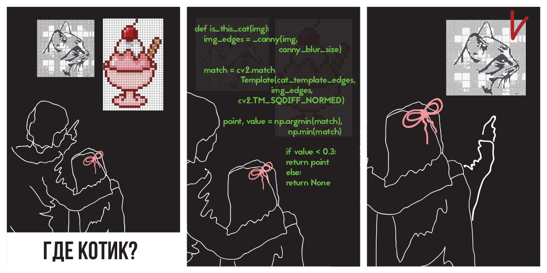
Finding objects in the pictures
We are engaged in the purchase of traffic from Adwords (advertising platform from Google). One of the regular tasks in this area is the creation of new banners. Tests show that banners lose effectiveness over time, as users get used to the banner; Seasons and trends are changing. In addition, we have a goal to capture different niches of the audience, and narrowly targeted banners work better.
In connection with the release of new countries, the question of the localization of banners became acute. For each banner it is necessary to create versions in different languages and with different currencies. You can ask designers to do this, but this manual work will add additional burden on the already scarce resource.
It looks like a task that is easy to automate. To do this, it is enough to make a program that will impose on the banner of a banner a localized price for the “price tag” and call to action (a phrase like “buy now”) on the button. If the printing of text on a picture is easy to implement, then determining the position where to put it is not always trivial. Peppercorn adds that the button comes in different colors, and is slightly different in shape.
This article is devoted to: how to find the specified object in the picture? Popular methods will be parsed; given the scope, features, pros and cons. These methods can be used for other purposes: developing programs for surveillance cameras, automating UI testing, and the like. The described difficulties can be met in other tasks, and the techniques used are used for other purposes. For example, the Canny Edge Detector is often used to pre-process images, and the number of key points (keypoints) can be used to assess the visual “complexity” of an image.
I hope that the described solutions will replenish your arsenal of tools and tricks for solving problems.
The code is shown in Python 3.6 ( repository ); OpenCV library required. The reader is expected to understand the basics of linear algebra and computer vision.
We will focus on finding the button itself. We will remember about finding price tags (since finding a rectangle can be solved in more simple ways), but we will omit it, since the solution will look the same way.
Template matching
The very first thought that comes to mind is, why not just take and find in the picture the region that most resembles a button in terms of the difference in pixel colors? This makes template matching, a method based on finding a place in an image that is most similar to a template. The “similarity” of an image is defined by a certain metric. That is, the pattern is "superimposed" on the image, and the discrepancy between the image and the pattern is considered. The position of the template, in which this discrepancy will be minimal, and will mean the place of the desired object.
As a metric, you can use different options, for example - the sum of squared differences between the template and the picture (sum of squared differences, SSD), or use cross-correlation (CCORR). Let f and g be an image and a pattern of dimensions (k, l) and (m, n), respectively (for the time being, we will ignore the color channels); i, j is the position on the image to which we have "attached" the template.
S S D i , j = s u m a = 0 .. m , b = 0 .. n ( f i + a , j + b - g a , b ) 2
CCORRi,j= suma=0..m,b=0..n(fi+a,j+b cdotga,b)2
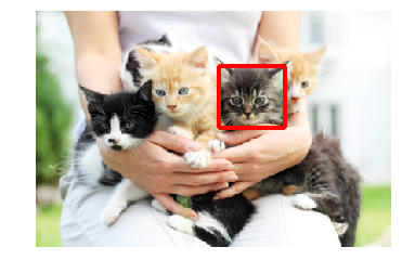
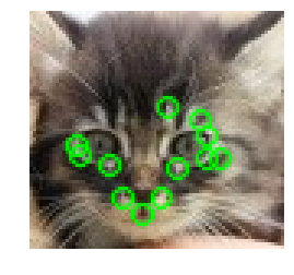
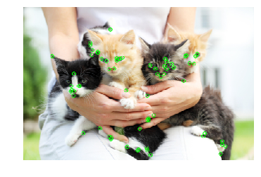
Let's try to apply the difference of squares to find a kitten
On the picture
(Picture taken from PETA Caring for Cats).
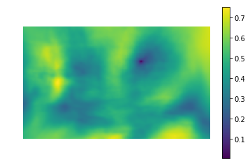
The left picture is the metric values of space similarity in the picture to the template (i.e. SSD values for different i, j). The dark area is the place where the difference is minimal. This is the pointer to the place that most closely resembles the pattern - this place is circled in the right picture.
Cross-correlation is actually a convolution of two images. Convolutions can be implemented quickly using the fast Fourier transform. According to the convolution theorem, after the Fourier transform, the convolution turns into a simple elementwise multiplication:
CCORRi,j=f circledastg=IFFT(FFT(f circledastg))=IFFT(FFT(f) cdotFFT(g))
Where circledast - convolution operator. Thus, we can quickly calculate the cross-correlation. This gives the total complexity O (kllog (kl) + mnlog (mn)) , versus O (klmn) when implemented head-on. The difference square can also be realized using convolution, since after opening the brackets it will turn into the difference between the sum of squares of the image pixel values and cross-correlation:
SSDi,j= suma=0..m,b=0..n(fi+a,j+b−ga,b)2=
= suma=0..m,b=0..nf2i+a,j+b−2fi+a,j+bga,b+g2a,b=
= suma=0..m,b=0..nf2i+a,j+b+g2a,b−2CCORi,j
Details can be found in this presentation .
We turn to the implementation. Fortunately, colleagues from Intel's Nizhny Novgorod department took care of us by creating the OpenCV library, it already implemented a template search using the matchTemplate method (by the way, the FFT implementation is used, although the documentation does not mention it anywhere):
- CV_TM_SQDIFF - the sum of squares of differences in pixel values
- CV_TM_SQDIFF_NORMED - the sum of the square of color differences, normalized to the range of 0..1.
- CV_TM_CCORR - the sum of the element by element works of the pattern and the segment of the picture
- CV_TM_CCORR_NORMED is the sum of the elementwise products, normalized to the range -1..1.
- CV_TM_CCOEFF - cross-correlation of images without an average
- CV_TM_CCOEFF_NORMED - cross-correlation between images without an average, normalized to -1..1 (Pearson correlation)
Apply them to search for a kitten:
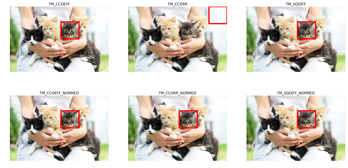
It can be seen that only TM_CCORR did not cope with its task. This is understandable: since it is a scalar product, the highest value of this metric will be when comparing the template with a white rectangle.
You may notice that these metrics require pixel-by-pixel matching of the pattern in the search image. Any deviation of gamma, light or size will cause the methods to not work. Let me remind you that this is our case: the buttons can be of different sizes and different colors.
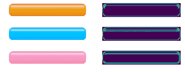
The problem of different colors and light can be solved by applying the edge detection filter. This method leaves only information about where in the image were sharp drops of color. Apply the Canny Edge Detector (we'll take a closer look at it in more detail) to the buttons of different colors and brightness. On the left are the original banners, and on the right the result of applying the Canny filter.
In our case, there is also a problem of different sizes, but it has already been solved. The log-polar transformation transforms the image into a space in which the change in scale and rotation will appear as an offset. Using this transformation, we can restore the scale and angle. After that, having scaled and rotated the template, you can also find the position of the template on the original image. FFT can also be used throughout this procedure, as described in An FFT-Based Technique for Translation, Rotation, and Scale-Invariant Image Registration . In the literature, the case is considered when the template varies horizontally and vertically proportionally, and at the same time the scale factor varies within small limits (2.0 ... 0.8). Unfortunately, resizing a button can be larger and disproportionate, which can lead to an incorrect result.
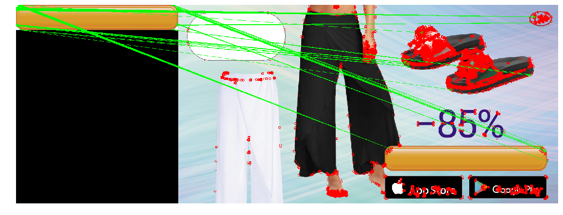
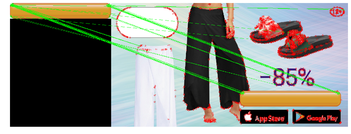
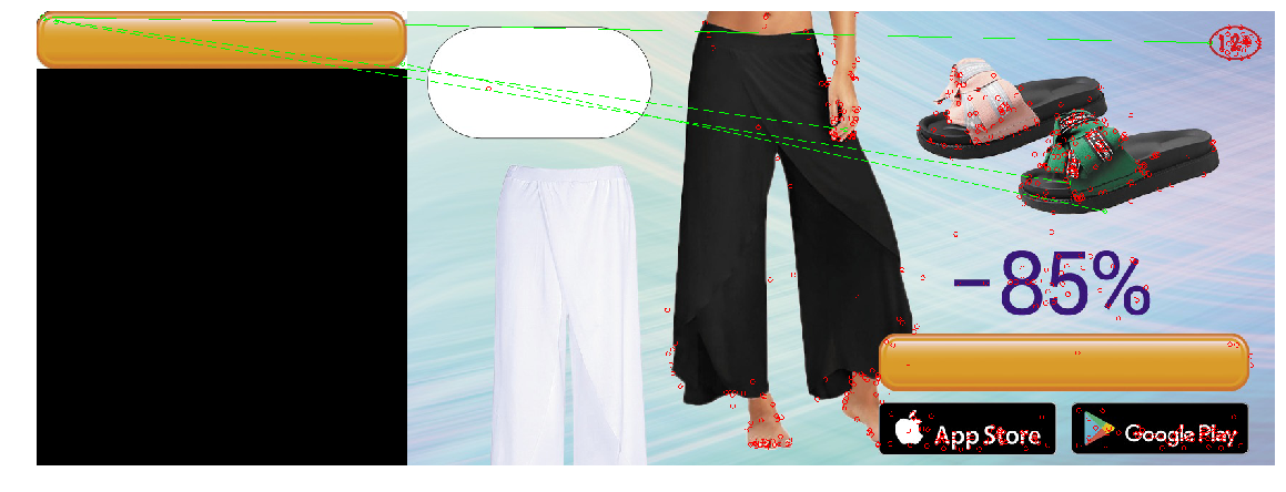
Apply the resulting construction (Canny filter, restoring only the scale through the log-polar transformation, obtaining the position through finding a place with the minimum quadratic difference), to find the button in the three pictures. We will use the big yellow button as a template:

At the same time, the banners on the buttons will be of different types, colors and sizes:

In the case of resizing the button, the method did not work correctly. This is due to the fact that the method involves changing the size of the buttons in the same number of times both horizontally and vertically. However, this is not always the case. On the right picture, the size of the button vertically has not changed, but horizontally it has decreased greatly. If the size of the image is too large, the distortions caused by the log-polar transformation make the search unstable. In this regard, the method could not detect the button in the third case.
Keypoint detection
You can try a different approach: instead of looking for the button as a whole, let's find its typical parts, for example, the corners of the button, or the elements of the border (there is a decorative stroke along the contour of the button). It seems that finding corners and curbs is easier, since these are small (and therefore simple) objects. What lies between the four corners and the border - and will be a button. The class of methods for finding key points is called “keypoint detection”, and the algorithms for comparing and searching images using key points are called “keypoint matching”. The search for a pattern in a picture comes down to applying the algorithm for finding key points to a pattern and a picture, and comparing key points of a pattern and picture.
Usually “cue points” are found automatically, finding the pixels whose surroundings have certain properties. It was invented many ways and criteria for their location. All these algorithms are heuristics, which find some characteristic elements of the image, as a rule - angles or sharp drops in color. A good detector should work quickly and be resistant to image transformations (when changing the image, key points should not cease to be / move).
Harris corner detector
Harris corner detector is considered one of the most basic algorithms. For the picture (here and below, we believe that we operate with “intensity” —the image translated in grayscale), he tries to find points in the vicinity of which the intensity drops are more than a certain threshold. The algorithm looks like this:
From intensity I are the derivatives along the X and Y axis ( Ix and Iy respectively). They can be found, for example, by applying a Sobel filter.
For a pixel count square Ix square Iy and works Ix and Iy . Some sources refer to them as Ixx , Ixy and Ixy - which does not add clarity, as you might think that these are the second derivatives of the intensity (and this is not so).
For each pixel, we count the sums in a certain neighborhood (more than 1 pixel) w the following characteristics:
A= sumx,yw(x,y)IxIx
B= sumx,yw(x,y)IxIy
C= sumx,yw(x,y)IyIy
As in Template Detection, this procedure for large windows can be carried out efficiently by using the convolution theorem.For each pixel count the value star heuristics r
R=Det(H)−k(Tr(H))2=(AB−C2)−k(A+B)2
Value k is chosen empirically in the range [0.04, 0.06] If R at some pixel is greater than a certain threshold, then the neighborhood w This pixel contains an angle, and we mark it as a key point.The previous formula can create clusters of key points lying next to each other, in which case it is worthwhile to remove them. This can be done by checking for each point whether its value is R maximum among immediate neighbors. If not, then the key point is filtered out. This procedure is called non-maximum suppression .
star Formula R so chosen for a reason. A,B,C - components of the structural tensor - matrices describing the behavior of the gradient in the neighborhood:
H = \ begin {pmatrix} A & C \\ C & B \ end {pmatrix}
This matrix is in many properties and form similar to the covariance matrix. For example, they are both positive semidefinite matrices, but the similarity is not limited to this. Let me remind you that the covariance matrix has a geometric interpretation. The eigenvectors of the covariance matrix indicate the directions of the greatest variance of the input data (on which the covariance was calculated), and the eigenvalues, the spread along the axis:

The picture is taken from http://www.visiondummy.com/2014/04/geometric-interpretation-covariance-matrix/
The eigenvalues of the structure tensor behave in the same way: they describe the scatter of gradients. On a flat surface, the eigenvalues of the structural tensor will be small (because the spread of the gradients themselves will be small). The eigenvalues of the structural tensor, built on a piece of a picture with a face, will vary greatly: one number will be large (and correspond to its own vector, directed perpendicular to the face), and the second will be small. On the angle tensor, both eigenvalues will be large. Based on this, we can build a heuristic ( lambda1, lambda2 - eigenvalues of the structure tensor).
R= lambda1 lambda2−k( lambda1+ lambda2)2
The value of this heuristic will be large when both eigenvalues are large.
The sum of the eigenvalues is the trace of the matrix, which can be calculated as the sum of the elements on the diagonal (and if you look at formulas A and B, it becomes clear that this is also the sum of the squares of gradient lengths in the region):
lambda1+ lambda2=Tr(H)=A+B
The product of the eigenvalues is the determinant of the matrix, which in the case of 2x2 is also easy to write:
lambda1 lambda2=Det(H)=AB−C2
Thus, we can effectively calculate R , expressing it in terms of the components of the structural tensor.
FAST
Harris's method is good, but there are many alternatives to it. We will not consider everything in the same way as the method above; we will mention only a few popular ones in order to show interesting techniques and compare them in action.

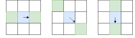
Pixels checked by the FAST algorithm
An alternative to the Harris method is FAST . As the name suggests, FAST is much faster than the method described above. This algorithm tries to find points that lie on the edges and corners of objects, i.e. in places of differential contrast. Their finding is as follows: FAST builds a circle of radius R around the candidate pixel and checks whether there is a continuous segment of pixels of length t that is darker (or lighter) than the candidate pixel by K units. If this condition is met, then the pixel is considered a “key point”. With certain t, we can implement this heuristic effectively by adding a few preliminary checks that will cut off the pixels of guaranteed non-angles. For example, when R=3 and t=$1 , it is enough to check if there are 3 consecutive pixels among the 4 extreme pixels that are strictly darker / brighter than the center on K (in the picture - 1, 5, 9, 13). This condition allows you to effectively cut off candidates that are not exactly key points.
SIFT
Both previous algorithms are not resistant to changes in the size of the image. They do not allow to find the pattern in the picture, if the scale of the object has been changed. SIFT (Scale-invariant feature transform) offers a solution to this problem. Take an image from which we extract the key points, and begin to gradually reduce its size with some small step, and for each scale option we will find key points. Scaling is a hard procedure, but a decrease of 2/4/8 / ... can be done efficiently by skipping pixels (in SIFT, these multiple scales are called “octaves”). Intermediate scales can be approximated by applying Gaussian blur with different core sizes to the image. As we have already described above, this can be done computationally efficiently. The result will be similar to if we first reduced the image, and then increased it to its original size - small details are lost, the image becomes “zamylennym”.
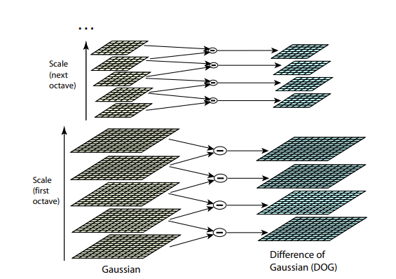
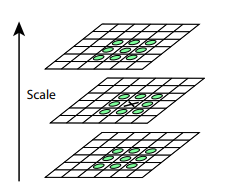
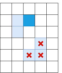
After this procedure, we calculate the difference between neighboring scales. Large (by module) values in this difference will be obtained if some small detail ceases to be visible at the next scale level, or, on the contrary, the next scale level starts to capture some detail that was not visible at the previous one. This technique is called DoG, Difference of Gaussian. We can assume that a large value in this difference is already a signal that there is something interesting in this place on the image. But we are interested in the scale for which this key point will be the most expressive. For this, we will consider a key point not only a point that differs from its environment, but also differs most of all among the different scales of images. In other words, we will choose the key point not only in the space X and Y, but in the space (X,Y,Scale) . In SIFT, this is done by finding points in the DoG (Difference of Gaussians), which are local maxima or minima in 3x3x3 cube of space (X,Y,Scale) around her:
Algorithms for finding key points and constructing SIFT and SURF descriptors are patented. That is, for their commercial use, you must obtain a license. That is why they are not available from the main opencv package, but only from a separate opencv_contrib package. However, so far our research is purely academic in nature, so nothing prevents us from participating in SIFT in comparison.
Descriptors
Let's try to apply some kind of detector (for example, Harris) to the template and the picture.
After finding the key points in the picture and the template, you need to somehow compare them with each other. Let me remind you that we have so far extracted only the positions of key points. What this point means (for example, in which direction the angle found is directed), we have not yet determined. And such a description can help in matching the points of the image and the pattern with each other. Some of the points of the pattern in the picture can be shifted by distortions, closed by other objects, so relying solely on the position of the points relative to each other seems to be unreliable. Therefore, for each key point, let's take its neighborhood in order to construct a certain description (descriptor), which then allows us to take a couple of points (one point from the template, one of the picture), and compare their similarities.
BRIEF
If we make a descriptor in the form of a binary array (i.e., an array of 0 and 1), then we will be able to compare them extremely effectively by making XOR two descriptors, and count the number of ones as a result. How to make such a vector? For example, we can select N pairs of points in the vicinity of a key point. Then, for the i-th pair, check whether the first point is brighter than the second, and if so, write 1 in the i-th position of the descriptor. Thus, we can create an array of length N. If we choose as one of the points of all pairs If there is any single point in the neighborhood (for example, the center of the neighborhood is the key point itself), then such a descriptor will be unstable to noise: just enough to change the brightness of just one pixel to make the entire descriptor go. The researchers found that it is sufficient to efficiently select points randomly (from a normal distribution with a center at a key point). This is the basis of the BRIEF algorithm.

Part of the methods considered by the authors for generating pairs. Each segment symbolizes a pair of generated points. The authors found that the GII option works slightly better than the other options.
After we have chosen pairs, they should be fixed (that is, they should not be generated every time the descriptor is started, but generated once and remembered). In the implementation from OpenCV, these pairs are generated beforehand and hard-coded .
SIFT Descriptor
SIFT can also efficiently read descriptors using the results of applying Gaussian blur on different octaves in the picture. To calculate the descriptor, SIFT selects a 16x16 region around a key point, and breaks it into blocks of 4x4 pixels. For each pixel, a gradient is considered (we operate on the same scale and octave at which the key point was found). Gradients in each block are divided into 8 groups in the direction (up, up, right, right, etc.). In each group the lengths of the gradients are added up - 8 numbers are obtained, which can be represented as a vector describing the direction of the gradients in the block. This vector is normalized for resistance to changes in brightness. So, for each block, an 8-dimensional vector of unit length is calculated. These vectors are concatenated into one large descriptor of length 128 (in a neighborhood of 4 * 4 = 16 blocks, each with 8 values). To compare the descriptors, the Euclidean distance is used.
Comparison
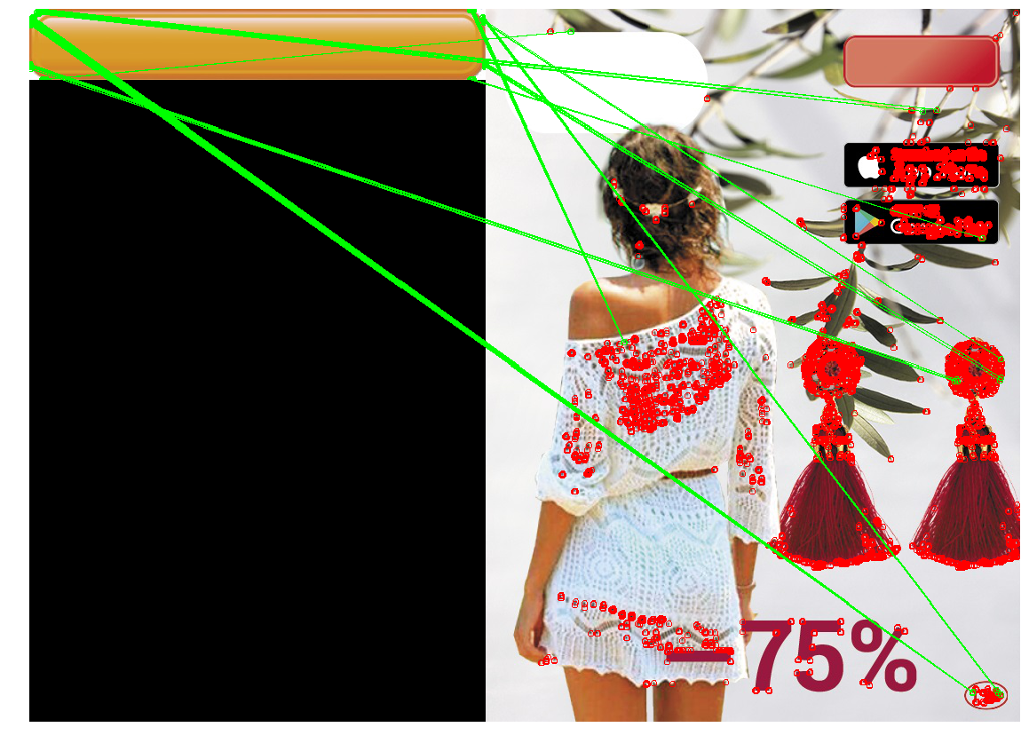
By finding the pairs of the most suitable key points for each other (for example, making pairs eagerly, starting with the most descriptors), we can finally compare the pattern and the picture:
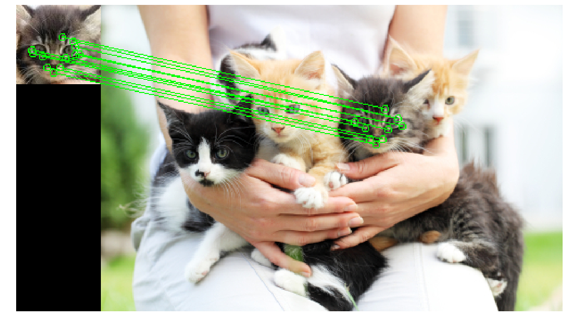
The cat was found - but here we have a pixel-by-pixel correspondence between the template and the fragment of the picture. And what will happen in the case of a button?
Suppose we have a rectangular button. If the key point is located on the corner, then three-quarters of the locale of the point will be exactly what lies outside the button. And what lies outside the button varies greatly from image to image, depending on what the button is on top of. What proportion of the descriptor will remain constant when the background changes? In the BRIEF descriptor, since the coordinates of a pair are chosen randomly and independently in the locale, the descriptor bit will remain constant only when both points lie on the button. In other words, in BRIEF only 1/16 of the descriptor will not change. In SIFT, the situation is slightly better - due to the block structure, the of the descriptor will not change.
In this regard, we will continue to use the SIFT descriptor.
Detector Comparison
Now apply all the knowledge gained to solve our problem. : , . .
| Harris corner detector | FAST | SIFT |
|---|---|---|
 |  |  |
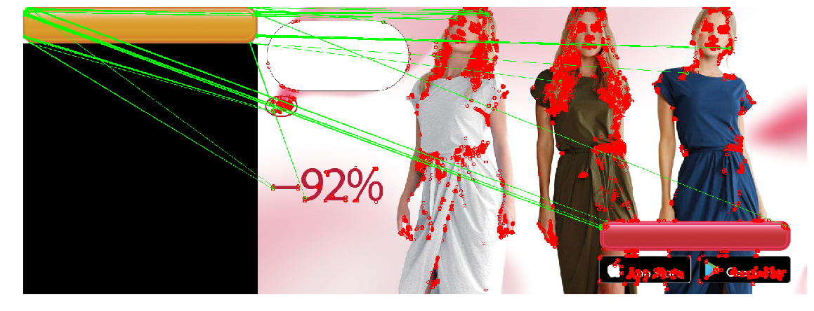 | 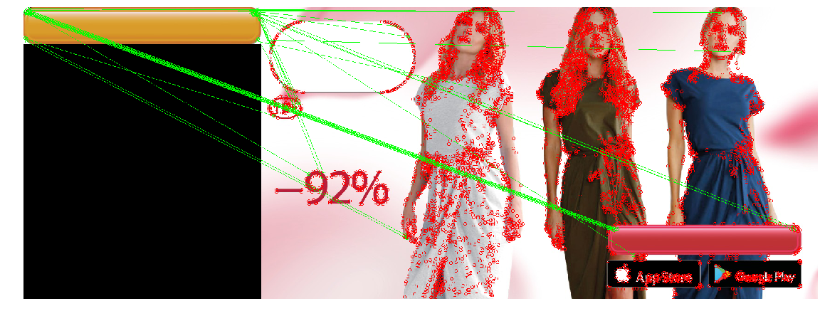 | 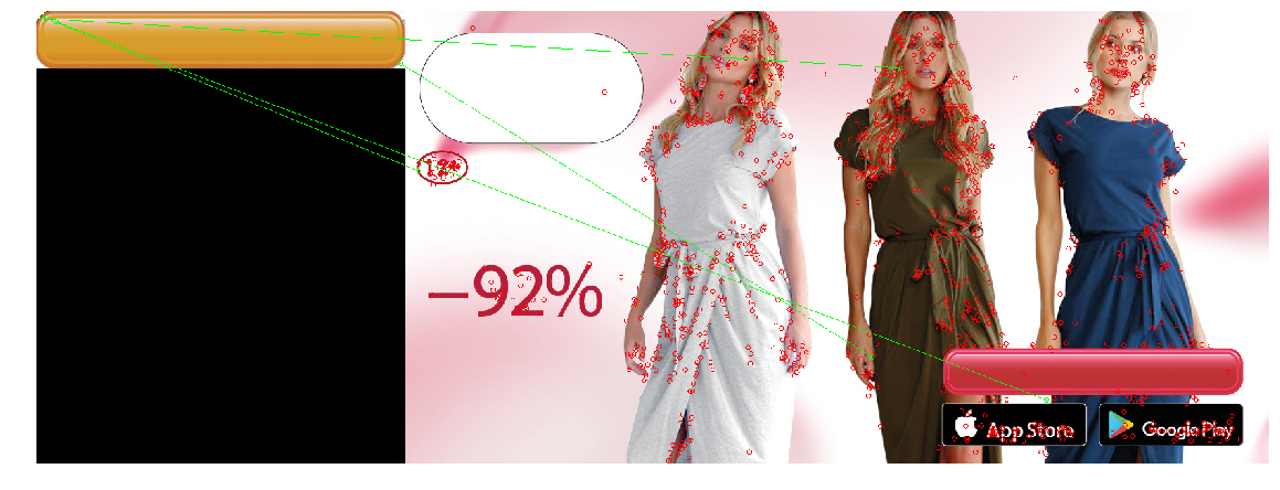 |
 | 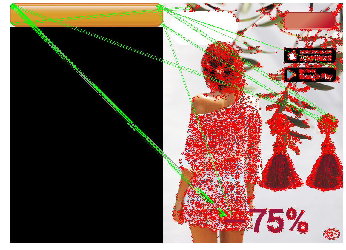 | 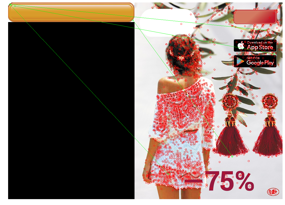 |
SIFT . — , .
, . . , , , , . , , () . . , (, , ) , . , . - : , .
— , , , , ( , , ). , , "", , . , " " .
, . , , , , . ( , ) , , . , , — , , , . :
Contour detection
— - ( — ), . (/edges), , . contour detection.
Edge detection
keypoint detection, -, . , . , Harris corner detector. Ix and Iy . , — : Il=I2x+I2y (, Tr(H) , ). , , Il ( non-maximum suppression), 8 , 8, I, :
, — I. — , non-maximum suppression.
, . , non-maximum suppression , .
, non-maximum suppression , - , Il. “double thresholding”: Il, , Low, High “ ”. , Low High, “ ”, “ ”:
- “ ”, - — . , .
Canny Edge Detector. , .
Border tracking
— . ( , ), , . non-maximum suppression Canny, , , . , , -, “”. , ( ), ( , - ):

border tracking, (, , ), . , .
, — ? > , . “” , , , . , — . , contour matching , — , ( ). , . , :
- ( 100 )
- . 0.8, — , 20% — .
, , , . Canny , , - .
:
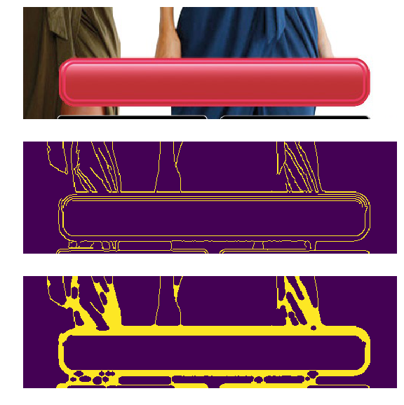
Canny filter (2 ) , - , - non-max suppression . (3 ) .
. , , . , . , .
|  |
|  |
|  |
|
. , (1 ~20) iOS Appstore Google Apps, ( ). , .
Conclusion
Let's sum up.“Classic” CV without deep learning still works, and on its basis it is possible to solve problems. They are unpretentious and do not require a large amount of labeled data, powerful iron, and they are easier to debug. However, they introduce additional assumptions, and therefore with their help not every problem can be solved effectively.
- Template Matching is the easiest way, based on finding a place in an image that is most similar (by some simple metric) to a template. Efficient with pixel matching. You can make it resistant to turns and small changes in size, but with large changes it may not work correctly.
- Keypoint detection / matching - find the key points, match the points of the image and the pattern. The detectors are resistant to turns, changes in scale (depending on the detector and descriptor selected), and the comparison is resistant to partial overlaps. But this method works well only if there are enough "key points" in the object, and the locales of the pattern and image points match quite well (that is, the same object is in the pattern and image).
- Contour detection - finding the contours of objects, and finding a contour similar to the contour of the desired object. This solution takes into account only the shape of the object, and ignores its content and color (which can be both a plus and a minus).
An informed reader may notice that our task can be solved with the help of modern, trained computer vision methods. For example, the YOLO network returns the bounding box of the desired object — namely, that is what interests us. Yes, we successfully tested and launched a solution based on deep learning - but as a second iteration (already after the localization tool was launched and started working). These solutions are more resistant to changes in the parameters of the buttons, and have many positive properties: for example, instead of manually selecting thresholds and parameters, you can simply add to the training set examples of banners on which the network is mistaken (Active Learning). Using deep learning for our task has its own problems and interesting points. For example - many modern computer vision methods require a large number of labeled images, and we had no markup (as in many real cases), and the total number of different banners does not exceed several thousand. Therefore, we decided to mark out a small number of images ourselves, and write a generator that will create other similar banners based on them. There are many interesting tricks in this direction. There are many other pitfalls, and the very task of determining the position of the computer vision object is extensive, and has many ways to solve it. Therefore, it was decided to limit the field of view of the article, and decisions based on in-depth training were not considered.
Code with notebooks that implement the described methods and draw pictures of the article can be found in the repository ).
')
Source: https://habr.com/ru/post/445354/
All Articles