Delaunay triangulation algorithm using the sweeping line method
Good day!
In this article I will describe in detail the algorithm that I got as a result of using the idea of a “sweeping line” to construct the Delaunay triangulation on the plane. There are several ideas in it that I have never met anywhere when I read articles about triangulation.
Perhaps someone will also find them unusual. I will try to do everything in the best traditions and include the following things in the story: a description of the data structures used, a description of the steps of the algorithm, proof of correctness, time estimates, and a comparison with an iterative algorithm using a kD-tree.
It is said that triangulation is given on the set of points on the plane, if some pairs of points are connected by an edge, any end face in the resulting graph forms a triangle, the edges do not intersect, and the graph is maximal in the number of edges.
')
Delaunay triangulation is such a triangulation in which for any triangle it is true that there are no points from the original set inside the circle described around it.
Note : for a given set of points in which no 4 points are on the same circle, there is exactly one Delaunay triangulation.
Let triangulation be given on a set of points. We say that a certain subset of points satisfies the Delone condition if the triangulation bounded on this subset is a Delaunay triangulation for it.
The fulfillment of the Delaunay condition for all points forming a quadrilateral in triangulation is equivalent to the fact that this triangulation is a Delaunay triangulation.
Note : for nonconvex quadrilaterals, the Delone condition is always satisfied, and for convex quadrangles (whose vertices do not lie on one circle) there are exactly 2 possible triangulations (one of which is the Delaunay triangulation).
The task is to construct a Delaunay triangulation for a given set of points.
Let a minimal convex hull (further MBO) of a finite set of points (edges connecting some of the points so that they form a polygon containing all points of the set) and a point A outside the shell be given. Then the point of the plane is called visible for point A, if the segment connecting it with point A does not intersect the MBO.
The edge of the MVO is said to be visible for point A if its ends are visible for A.
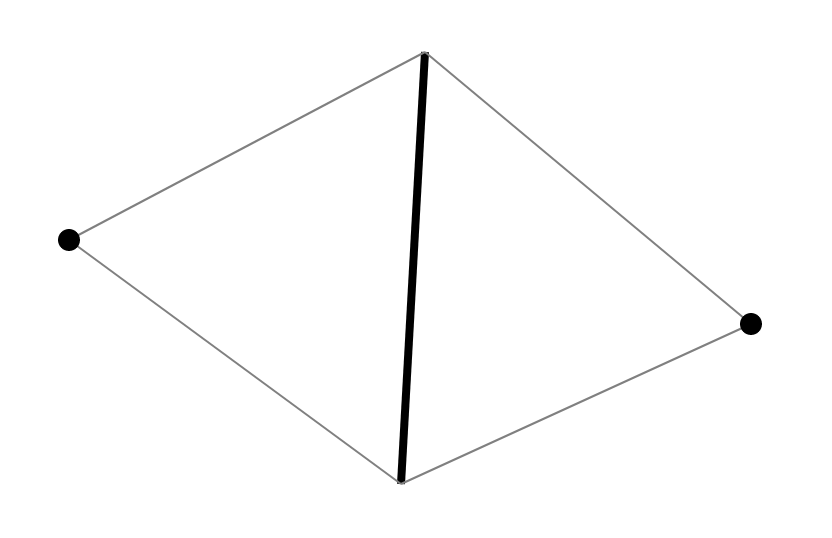
In the following image, the edges visible for the red dot are marked in red:
Note : the Delaunay triangulation contour is the MVO for the points on which it is built.
Note 2 : in the algorithm, the edges visible for the added point A form a chain, that is, several successive edges of the MVO
There are some standard methods, well described in the book Skvortsova [1]. Due to the specifics of the algorithm, I will offer my version. Since I want to check the 4-gons on the Delone condition, we consider their structure. Each 4-gon in triangulation consists of 2 triangles with a common edge. Each edge has exactly 2 triangles adjacent to it. Thus, each quadrilateral in triangulation is generated by an edge and two vertices located opposite the edge in adjacent triangles.
Since two triangles and their adjacency are reconstructed along the edge and two vertices, we can restore triangulation in all such structures. Accordingly, it is proposed to store an edge with two vertices in the set and perform a search by edge (an ordered pair of vertices).
The idea of a sweeping straight line is that all points are sorted in one direction, and then processed in turn.
Note : in step (4) with a recursive start, you can not check the quadrilaterals generated by the edges emanating from the point considered at this iteration (there are always two of four). Most often they will be non-convex, for convex proof is purely geometric, I leave it to the reader. Further, we assume that only 2 recursive starts are performed for each rebuild.
Methods for checking quadrilaterals on the Delone condition can be found in the same book [1]. I will only note that when choosing a method with trigonometric functions, if there is an inaccurate implementation, negative sine values can be obtained, it makes sense to take them modulo.
It remains to understand how to effectively find the visible edges. Note that the previous added point S is in the MBO at the current iteration, since it has the greatest coordinate , and also visible for the current point. Then, noting that the ends of the visible edges form a continuous chain of visible points, we can go from point S in both directions along the MVO and collect the edges while they are visible (the visibility of the edge is checked using the vector product). Thus, it is convenient to store the MBO as a doubly linked list, at each iteration removing visible edges and adding 2 new ones from the point in question.
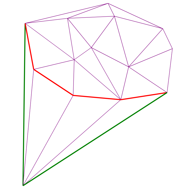
Two red dots - added and previous. The red edges at each moment make up the recursion stack from step (4):
To prove the correctness of the algorithm, it suffices to prove the invariant is preserved in steps (3) and (4).
After step (3), obviously, we get some triangulation of the current set of points.
In the process of executing step (4), all quadrangles that do not satisfy the Delone condition are on the recursion stack (follows from the description), which means that at the end of step (4), all quadrangles satisfy the Delaunay condition, that is, the Delaunay triangulation is indeed constructed. Then it remains to prove that the process in step (4) will ever end. This follows from the fact that all edges added during rebuilding come from the current vertex under consideration (that is, in the step they are no more than ) and from the fact that after adding these edges we will not consider quadrilaterals generated by them (see previous remark), and therefore, we add no more than once.
On average, on a uniform, normal distribution, the algorithm works quite well (the results are given below in the table). There is an assumption that his time is . In the worst case, there is an estimate. .
Let's look at the time of work in parts and understand which of them has the greatest impact on the final time:
For sorting we will use the estimate .
To begin with, we show that the total time spent searching for visible edges is . Note that at each iteration we find all visible edges and another 2 (the first not visible) in linear time. In step (3) we add new 2 edges to the MVO. Thus, in all, in the changing for the duration of the MBO algorithm, no more than edges, which means that there will be no more visible edges . We will also find edges that are not visible. Thus, in total there will be no more edges that corresponds to the time .
The total time to build triangles from step (3) with visible edges already found, obviously .
It remains to deal with step (4). First, we note that checking the Delone condition and rebuilding if it is not fulfilled are quite expensive actions (although they work for ). Only on checking the condition of Delone can take about 28 arithmetic operations. Let's look at the average number of rebuilds during this step. Practical results on some distributions are given below. For them, I really want to say that the average number of rebuilds grows at a logarithmic speed, but we will leave it as just an assumption.
Here I also want to note that the average number of rebuilds per point can vary greatly from the direction along which the sorting is performed. So on a million evenly distributed on a long low rectangle with an aspect ratio of 100,000: 1, this number varies from 1.2 to 24 (these values are achieved by sorting the data horizontally and vertically, respectively). Therefore, I see the sense to choose the direction of sorting in an arbitrary way (in this example, with an arbitrary choice, on average, there were about 2 rebuilds) or to select it manually if the data is known in advance.
Thus, the main time of the program usually takes a step (4). If it is performed quickly, then it makes sense to think about accelerating the sorting.
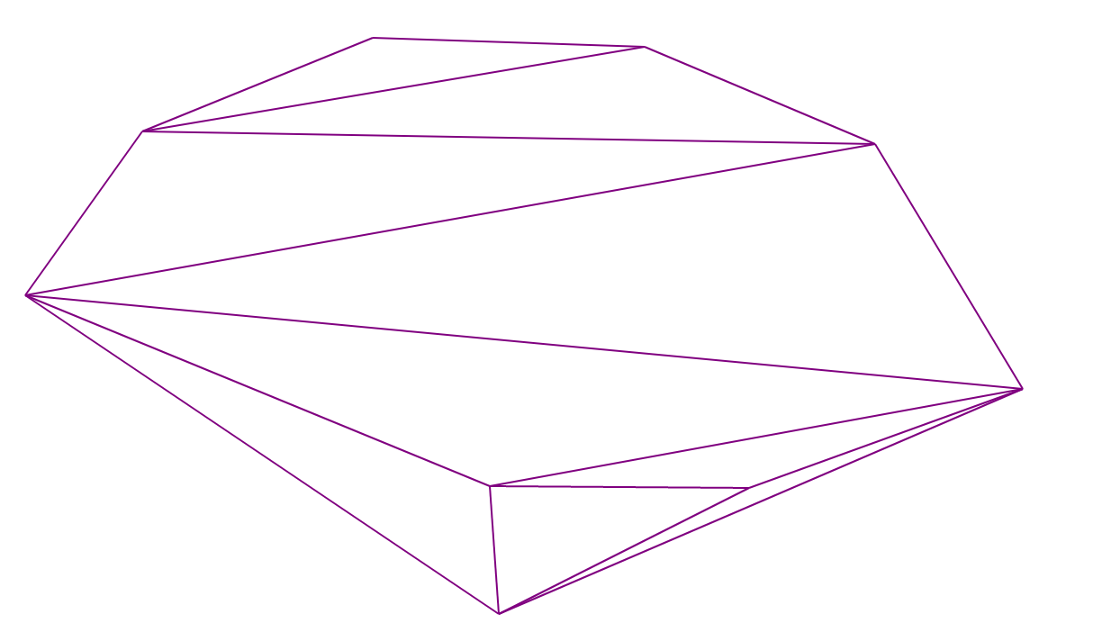
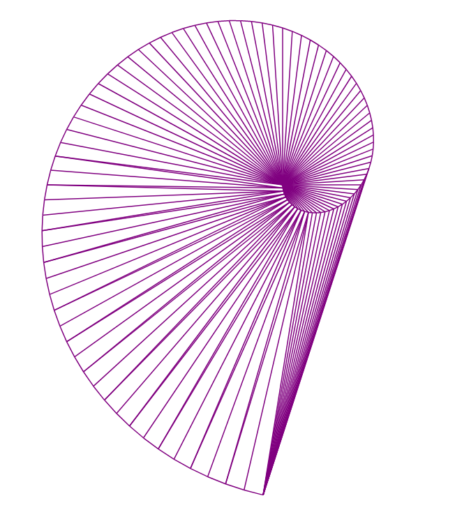
At worst on th iteration happens recursive call in step (4), that is, summing over all i, we get the asymptotics in the worst case . The following picture illustrates a beautiful example in which the program can work for a long time (1100 rebuildings on average when adding a new point with input data of 10,000 points).
I will briefly describe the above algorithm. When entering the next point with the help of a kD-tree (I advise you to read about it somewhere, if you do not know) we find a triangle already built close to it. Then by detour in depth we are looking for a triangle into which the point itself falls. We finish the edges at the vertices of the found triangle and actually perform step (4) from our algorithm for new quadrangles. Since a point can be outside of triangulation, for simplicity, it is proposed to cover all points with a large triangle (build it in advance), this will solve the problem.
In fact, if points are added in the order sorted by direction, then our algorithm actually works in the same way as iterative, except that the number of rebuilds is less. The following animation demonstrates this very well. The points on it were added from right to left, and all of them are covered with a large triangle, which is subsequently removed.
In an iterative algorithm, localization of a point (search for the desired triangle) occurs on average for , on the above distributions, on average, 3 rebuilds take place (as shown in [1]) under the condition of an arbitrary order of points supply. Thus, the sweeping straight line gains time from the iterative algorithm in localization, but loses it in rebuilds (which, I recall, are rather heavy). In addition, the iterative algorithm works online, which is also its distinguishing feature.
Here I just show some interesting triangulations resulting from the operation of the algorithm.
Here you can see an example of my code for this algorithm:
github.com/Vemmy124/Delaunay-Triangulation-Algorithm
Thanks for attention!
[1] Skvortsov A.V. Delaunay triangulation and its application. - Tomsk: Publishing house Tom. University, 2002. - 128 p. ISBN 5-7511-1501-5
In this article I will describe in detail the algorithm that I got as a result of using the idea of a “sweeping line” to construct the Delaunay triangulation on the plane. There are several ideas in it that I have never met anywhere when I read articles about triangulation.
Perhaps someone will also find them unusual. I will try to do everything in the best traditions and include the following things in the story: a description of the data structures used, a description of the steps of the algorithm, proof of correctness, time estimates, and a comparison with an iterative algorithm using a kD-tree.
Definitions and problem statement
Triangulation
It is said that triangulation is given on the set of points on the plane, if some pairs of points are connected by an edge, any end face in the resulting graph forms a triangle, the edges do not intersect, and the graph is maximal in the number of edges.
')
Delaunay triangulation
Delaunay triangulation is such a triangulation in which for any triangle it is true that there are no points from the original set inside the circle described around it.

Note : for a given set of points in which no 4 points are on the same circle, there is exactly one Delaunay triangulation.
Delone condition
Let triangulation be given on a set of points. We say that a certain subset of points satisfies the Delone condition if the triangulation bounded on this subset is a Delaunay triangulation for it.
Criterion for Delaunay Triangulation
The fulfillment of the Delaunay condition for all points forming a quadrilateral in triangulation is equivalent to the fact that this triangulation is a Delaunay triangulation.
Note : for nonconvex quadrilaterals, the Delone condition is always satisfied, and for convex quadrangles (whose vertices do not lie on one circle) there are exactly 2 possible triangulations (one of which is the Delaunay triangulation).
![]()
The task is to construct a Delaunay triangulation for a given set of points.
Algorithm Description
Visible points and visible edges
Let a minimal convex hull (further MBO) of a finite set of points (edges connecting some of the points so that they form a polygon containing all points of the set) and a point A outside the shell be given. Then the point of the plane is called visible for point A, if the segment connecting it with point A does not intersect the MBO.
The edge of the MVO is said to be visible for point A if its ends are visible for A.
In the following image, the edges visible for the red dot are marked in red:

Note : the Delaunay triangulation contour is the MVO for the points on which it is built.
Note 2 : in the algorithm, the edges visible for the added point A form a chain, that is, several successive edges of the MVO
Storage of triangulation in memory
There are some standard methods, well described in the book Skvortsova [1]. Due to the specifics of the algorithm, I will offer my version. Since I want to check the 4-gons on the Delone condition, we consider their structure. Each 4-gon in triangulation consists of 2 triangles with a common edge. Each edge has exactly 2 triangles adjacent to it. Thus, each quadrilateral in triangulation is generated by an edge and two vertices located opposite the edge in adjacent triangles.
Since two triangles and their adjacency are reconstructed along the edge and two vertices, we can restore triangulation in all such structures. Accordingly, it is proposed to store an edge with two vertices in the set and perform a search by edge (an ordered pair of vertices).
Algorithm
The idea of a sweeping straight line is that all points are sorted in one direction, and then processed in turn.
- Sort all points along some straight line (for simplicity by the coordinate ).
- Construct a triangle on the first 3 points.
Further, for each next point, we will perform steps that preserve the invariant that there is a Delaunay triangulation for already added points and, accordingly, an MBO for them. - Add the triangles formed by the visible edges and the point itself (that is, we add edges from the point in question to all the ends of the visible edges).
- Let us check on the Delone condition all quadrilaterals generated by visible edges. If somewhere the condition is not fulfilled, then we rebuild the triangulation in the quadrilateral (I remind you that there are only two) and recursively run the test for quadrilaterals generated by the edges of the current quadrilateral (because only in them after changing the Delone condition could be broken).
Note : in step (4) with a recursive start, you can not check the quadrilaterals generated by the edges emanating from the point considered at this iteration (there are always two of four). Most often they will be non-convex, for convex proof is purely geometric, I leave it to the reader. Further, we assume that only 2 recursive starts are performed for each rebuild.
Delone check
Methods for checking quadrilaterals on the Delone condition can be found in the same book [1]. I will only note that when choosing a method with trigonometric functions, if there is an inaccurate implementation, negative sine values can be obtained, it makes sense to take them modulo.
Search for visible edges
It remains to understand how to effectively find the visible edges. Note that the previous added point S is in the MBO at the current iteration, since it has the greatest coordinate , and also visible for the current point. Then, noting that the ends of the visible edges form a continuous chain of visible points, we can go from point S in both directions along the MVO and collect the edges while they are visible (the visibility of the edge is checked using the vector product). Thus, it is convenient to store the MBO as a doubly linked list, at each iteration removing visible edges and adding 2 new ones from the point in question.
The visualization of the algorithm
Two red dots - added and previous. The red edges at each moment make up the recursion stack from step (4):
Algorithm correctness
To prove the correctness of the algorithm, it suffices to prove the invariant is preserved in steps (3) and (4).
Step (3)
After step (3), obviously, we get some triangulation of the current set of points.
Step (4)
In the process of executing step (4), all quadrangles that do not satisfy the Delone condition are on the recursion stack (follows from the description), which means that at the end of step (4), all quadrangles satisfy the Delaunay condition, that is, the Delaunay triangulation is indeed constructed. Then it remains to prove that the process in step (4) will ever end. This follows from the fact that all edges added during rebuilding come from the current vertex under consideration (that is, in the step they are no more than ) and from the fact that after adding these edges we will not consider quadrilaterals generated by them (see previous remark), and therefore, we add no more than once.
Time complexity
On average, on a uniform, normal distribution, the algorithm works quite well (the results are given below in the table). There is an assumption that his time is . In the worst case, there is an estimate. .

Let's look at the time of work in parts and understand which of them has the greatest impact on the final time:
Sort by direction
For sorting we will use the estimate .
Search for visible edges
To begin with, we show that the total time spent searching for visible edges is . Note that at each iteration we find all visible edges and another 2 (the first not visible) in linear time. In step (3) we add new 2 edges to the MVO. Thus, in all, in the changing for the duration of the MBO algorithm, no more than edges, which means that there will be no more visible edges . We will also find edges that are not visible. Thus, in total there will be no more edges that corresponds to the time .
Building new triangles
The total time to build triangles from step (3) with visible edges already found, obviously .
Rebuilding triangulation
It remains to deal with step (4). First, we note that checking the Delone condition and rebuilding if it is not fulfilled are quite expensive actions (although they work for ). Only on checking the condition of Delone can take about 28 arithmetic operations. Let's look at the average number of rebuilds during this step. Practical results on some distributions are given below. For them, I really want to say that the average number of rebuilds grows at a logarithmic speed, but we will leave it as just an assumption.

Here I also want to note that the average number of rebuilds per point can vary greatly from the direction along which the sorting is performed. So on a million evenly distributed on a long low rectangle with an aspect ratio of 100,000: 1, this number varies from 1.2 to 24 (these values are achieved by sorting the data horizontally and vertically, respectively). Therefore, I see the sense to choose the direction of sorting in an arbitrary way (in this example, with an arbitrary choice, on average, there were about 2 rebuilds) or to select it manually if the data is known in advance.
Thus, the main time of the program usually takes a step (4). If it is performed quickly, then it makes sense to think about accelerating the sorting.
Worst case
At worst on th iteration happens recursive call in step (4), that is, summing over all i, we get the asymptotics in the worst case . The following picture illustrates a beautiful example in which the program can work for a long time (1100 rebuildings on average when adding a new point with input data of 10,000 points).
Comparison with an iterative algorithm for constructing a Delaunay triangulation using a kD-tree
Description of the iterative algorithm
I will briefly describe the above algorithm. When entering the next point with the help of a kD-tree (I advise you to read about it somewhere, if you do not know) we find a triangle already built close to it. Then by detour in depth we are looking for a triangle into which the point itself falls. We finish the edges at the vertices of the found triangle and actually perform step (4) from our algorithm for new quadrangles. Since a point can be outside of triangulation, for simplicity, it is proposed to cover all points with a large triangle (build it in advance), this will solve the problem.
Similarity of algorithms
In fact, if points are added in the order sorted by direction, then our algorithm actually works in the same way as iterative, except that the number of rebuilds is less. The following animation demonstrates this very well. The points on it were added from right to left, and all of them are covered with a large triangle, which is subsequently removed.

Algorithm Differences
In an iterative algorithm, localization of a point (search for the desired triangle) occurs on average for , on the above distributions, on average, 3 rebuilds take place (as shown in [1]) under the condition of an arbitrary order of points supply. Thus, the sweeping straight line gains time from the iterative algorithm in localization, but loses it in rebuilds (which, I recall, are rather heavy). In addition, the iterative algorithm works online, which is also its distinguishing feature.
Conclusion
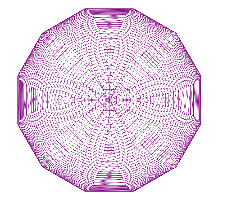
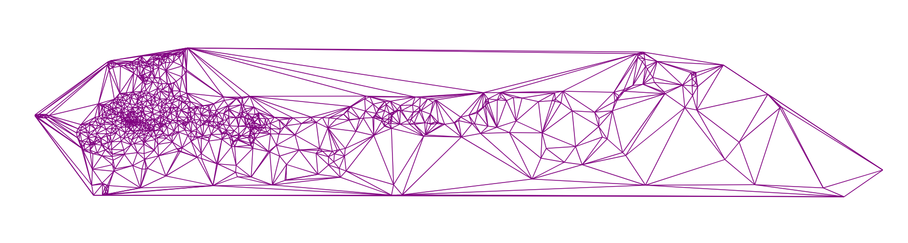
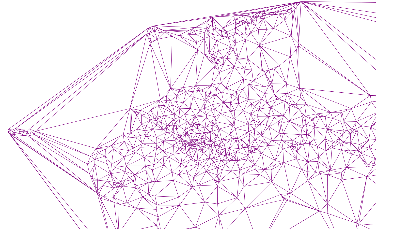
Here I just show some interesting triangulations resulting from the operation of the algorithm.
Beautiful pattern
Normal distribution, 1000 points

Uniform distribution, 1000 points

Triangulation, built on the locations of all cities of Russia
Here you can see an example of my code for this algorithm:
github.com/Vemmy124/Delaunay-Triangulation-Algorithm
Thanks for attention!
Literature
[1] Skvortsov A.V. Delaunay triangulation and its application. - Tomsk: Publishing house Tom. University, 2002. - 128 p. ISBN 5-7511-1501-5
Source: https://habr.com/ru/post/445048/
All Articles