Mountain Car: solve the classic problem with the help of training with reinforcements
As a rule, modifications of algorithms that rely on the features of a particular task are considered less valuable, since they are difficult to generalize to a wider class of problems. However, this does not mean that such modifications are not needed. Moreover, they can often significantly improve the result even for simple classical problems, which is very important in the practical application of algorithms. As an example in this post, I will solve the Mountain Car problem with the help of reinforcement training and show that using knowledge of how a problem is structured, it can be solved much faster.
My name is Oleg Svidchenko, now I study at the School of Physical-Mathematical and Computer Science of the St. Petersburg HSE, before that I had been studying at SPbAU for three years. I also work at JetBrains Research as a researcher. Before entering the university, I studied at the SSC of Moscow State University and became the winner of the All-Russian Olympiad in Informatics for Schoolchildren in the Moscow team.
If you are interested in trying out exercises with reinforcements, the Mountain Car challenge is great for this. Today, we will need Python with the Gym and PyTorch libraries installed, as well as basic knowledge of neural networks.
')
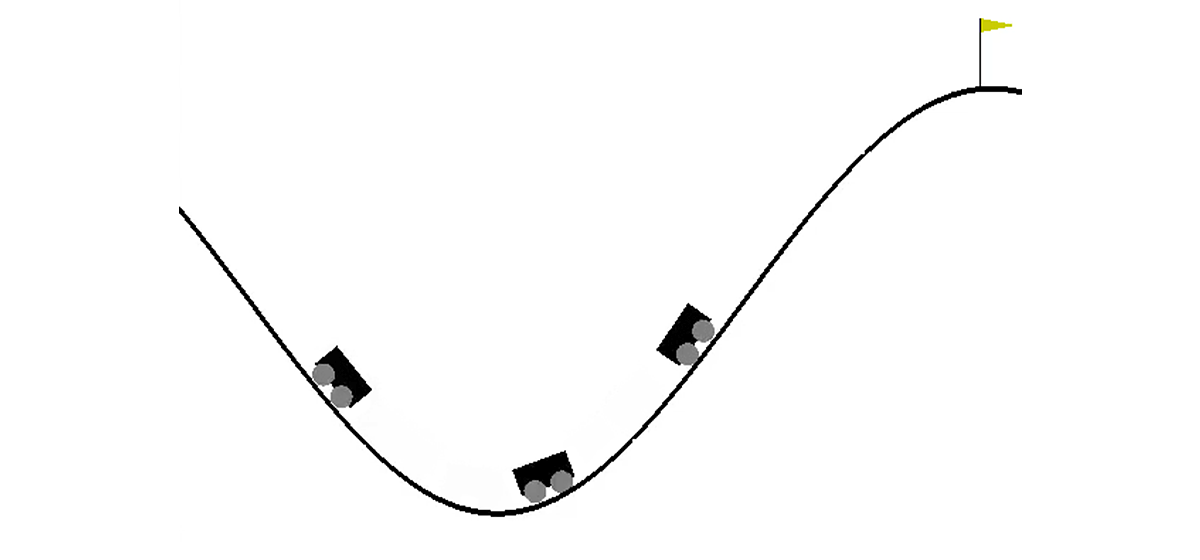
In a two-dimensional world, a car needs to climb from the depression between two hills to the top of the right hill. Everything is complicated by the fact that it does not have enough engine power to overcome the force of gravity and enter there at the first attempt. We are invited to train an agent (in our case, a neural network), who, while managing it, can climb the right hill as quickly as possible.
The machine is controlled through interaction with the medium. It is divided into independent episodes, and each episode is carried out step by step. At each step, the agent receives from the environment a state s and a reward r in response to the action he performed a . In addition, sometimes the medium may additionally report that the episode is over. In this task, s is a pair of numbers, the first of which is the position of the car on the curve (one coordinate is enough, since we cannot detach from the surface), and the second is its speed on the surface (with a sign). The reward r is a number, always equal to -1 for this task. Thus, we encourage the agent to complete the episode as quickly as possible. There are only three possible actions: push the car to the left, do nothing and push the car to the right. The numbers from 0 to 2 correspond to these actions. The episode can be completed if the car reaches the top of the right hill or if the agent has taken 200 steps.
On Habré there was already an article about DQN , in which the author described all the necessary theory quite well. Nevertheless, for the convenience of reading, I will repeat it here in a more formal form.
The learning task with reinforcement is given by a set of state space S, action space A, coefficient , transition functions T and reward functions R. In general, the transition function and the reward function can be random values, however, we now consider a simpler version in which they are uniquely defined. The goal is to maximize the cumulative reward. , where t is the step number in the environment, and T is the number of steps in the episode.
To solve this problem, we define the value-function V of the state s as the value of the maximum cumulative reward, provided that we start in the state s. Knowing such a function, we can solve the problem simply by moving each step to s with the maximum possible value. However, not everything is so simple: in most cases we do not know what action will lead us to the desired state. Therefore, we add the action a as the second parameter of the function. The resulting function is called the Q-function. It shows the maximum possible cumulative reward we can receive by performing the action a in the state s. But we can already use this function to solve the problem: being in the state s, we simply choose a such that Q (s, a) is maximal.
In practice, we do not know the real Q-function, but we can bring it closer using various methods. One such method is the Deep Q Network (DQN). His idea is that for each of the actions we approximate the Q-function using a neural network.
We now turn to practice. First we need to learn how to emulate the MountainCar environment. The Gym library will help us with this task, which provides a large number of standard environments for reinforcement learning. To create an environment, we need to call the make method of the gym module, passing it the name of the desired environment as a parameter:
Detailed documentation can be found here , and a description of the environment - here .
Let's take a closer look at what we can do with the environment we created:
DQN is an algorithm that uses a neural network to evaluate the Q-function. The original DeepMind article identified the standard architecture for Atari games using convolutional neural networks. Unlike these games, Mountain Car does not use the image as a state, so we’ll have to define the architecture ourselves.
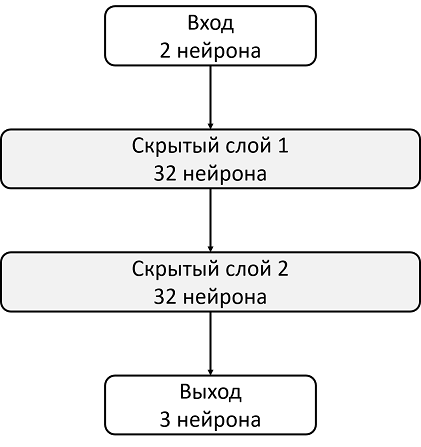
Take, for example, an architecture with two hidden layers of 32 neurons each. After each hidden layer, we will use ReLU as an activation function. Two numbers describing the state are fed to the input of the neural network, and at the output we get the estimate of the Q-function.
Since we will train the neural network on the GPU, we need to upload our network there:
The variable device will be global, since we also need to load the data.
We also need to define an optimizer that will update model weights using a gradient descent. Yes, there are more than one.
Now we will declare the function that will read the error function, the gradient along it, and apply the descent. But before that you need to download data from the batch to the GPU:
Next, we need to calculate the real values of the Q-function, but since we do not know them, we will evaluate them using the values for the following state:
And the current prediction:
Using target_q and q, we consider the loss function and update the model:
Since the model only considers the Q-function, and does not perform actions, we need to define a function that will decide which actions the agent will perform. As a decision-making algorithm, we take -greedy policy. Her idea is that the agent usually performs actions greedily, choosing the maximum of the Q function, however with probability he will perform a random act. Random actions are needed so that the algorithm can investigate those actions that it would not have committed guided only by greedy politics - this process is called exploration.
Since we use batchy for learning the neural network, we will need a buffer in which we will store the experience of interaction with the environment and from where we will choose batchy:
To begin with, we will declare constants that we will use in the learning process, and create a model:
Despite the fact that the interaction process would be logical to divide into episodes, to describe the learning process it is more convenient for us to divide it into separate steps, since we want to take one step of the gradient descent after each step of the environment.
Let's talk more about how one step of learning looks like. We will assume that we are now making a step with the step number from the max_steps steps and the current state. Then committing an action with -greedy policies would look like this:
Immediately add the experience to memory and start a new episode, if the current one is over:
And take a step gradient descent (if, of course, we can already collect at least one batch):
Now it remains to update target_model:
However, we would also like to follow the learning process. To do this, we will play an additional episode after each update of target_model with epsilon = 0, memorizing the total award in the rewards_by_target_updates buffer:
Run this code and get something like this:

Is this a bug? Is this the wrong algorithm? Are these bad options? Not really. In fact, the problem is in the task, namely in the function of the reward. Let's look at it more attentively. At each step, our agent receives a -1 reward, and this happens until the episode ends. This reward motivates the agent to complete the episode as quickly as possible, but at the same time does not tell him how to do it. Because of this, the only way to learn how to solve a problem in such a formulation for an agent is to solve it many times, using exploration.
Of course, one could try using more complex algorithms to explore the environment instead of our -greedy policies. However, firstly, because of their application, our model will become more complex, which we would like to avoid, and secondly, not the fact that they will work well enough for this task. Instead, we can eliminate the source of the problem by modifying the task itself, namely by changing the reward function, i.e. applying what is called reward shaping.
Our intuitive knowledge tells us that you need to accelerate to get on the hill. The greater the speed, the closer the agent is to the task. You can tell him about it, for example, by adding a speed module with some coefficient to the reward:
Accordingly, the line in the function fit
Here RS is short for Reward Shaping.
The progress is obvious: our agent obviously learned to drive up the hill, because the reward began to differ from -200. There is only one question left: if by changing the reward function, we changed the task itself, would the solution of the new problem we found be good for the old task?
To begin with, we will understand what “goodness” means in our case. Solving the problem, we are trying to find the optimal policy - one that maximizes the total reward for the episode. In this case, we can replace the word “good” with the word “optimal”, since we are looking for it. We also optimistically hope that our DQN will sooner or later find the optimal solution for the modified problem, and not get stuck in a local maximum. So, the question can be reformulated as follows: if by changing the reward function, we changed the task itself, would the optimal solution we found be optimal for the old problem?
As it turns out, we cannot provide such a guarantee in the general case. The answer depends on how we changed the function of the reward, how it was arranged earlier and how the environment itself is arranged. Fortunately, there is an article whose authors investigated how changing the reward function affects the optimality of the found solution.
First, they found a whole class of “safe” changes that are based on the potential method: where - potential, which depends only on the state. For such functions, the authors were able to prove that if the solution for the new problem is optimal, then for the old problem it is also optimal.
Second, the authors showed that for any other there is such a problem, the reward function R and the optimal solution of the modified problem, that this solution is not optimal for the original problem. This means that we cannot guarantee the goodness of the solution we found if we use a change that is not based on the method of potentials.
Thus, the use of potential functions to modify the reward function can only change the rate of convergence of the algorithm, but does not affect the final decision.
Now that we know how to safely change the reward, we will try to modify the task again using the potential method instead of naive heuristics:
Look at the graph of the original award:
As it turned out, in addition to the availability of theoretical guarantees, modification of the reward with the help of potential functions also significantly improved the result, especially in the early stages. Of course, there is a possibility that it would be possible to choose more optimal hyperparameters (random seed, gamma and other coefficients) for training the agent, however, reward shaping still significantly increases the rate of convergence of the model.
Thank you for reading to the end! I hope you enjoyed this small practice-oriented excursion to training with reinforcements. It is clear that Mountain Car is a “toy” task, however, as we could see, it can be difficult to teach an agent to solve even this seemingly simple task from a human point of view.
About myself
My name is Oleg Svidchenko, now I study at the School of Physical-Mathematical and Computer Science of the St. Petersburg HSE, before that I had been studying at SPbAU for three years. I also work at JetBrains Research as a researcher. Before entering the university, I studied at the SSC of Moscow State University and became the winner of the All-Russian Olympiad in Informatics for Schoolchildren in the Moscow team.
What do we need?
If you are interested in trying out exercises with reinforcements, the Mountain Car challenge is great for this. Today, we will need Python with the Gym and PyTorch libraries installed, as well as basic knowledge of neural networks.
')
Task Description
In a two-dimensional world, a car needs to climb from the depression between two hills to the top of the right hill. Everything is complicated by the fact that it does not have enough engine power to overcome the force of gravity and enter there at the first attempt. We are invited to train an agent (in our case, a neural network), who, while managing it, can climb the right hill as quickly as possible.
The machine is controlled through interaction with the medium. It is divided into independent episodes, and each episode is carried out step by step. At each step, the agent receives from the environment a state s and a reward r in response to the action he performed a . In addition, sometimes the medium may additionally report that the episode is over. In this task, s is a pair of numbers, the first of which is the position of the car on the curve (one coordinate is enough, since we cannot detach from the surface), and the second is its speed on the surface (with a sign). The reward r is a number, always equal to -1 for this task. Thus, we encourage the agent to complete the episode as quickly as possible. There are only three possible actions: push the car to the left, do nothing and push the car to the right. The numbers from 0 to 2 correspond to these actions. The episode can be completed if the car reaches the top of the right hill or if the agent has taken 200 steps.
Some theory
On Habré there was already an article about DQN , in which the author described all the necessary theory quite well. Nevertheless, for the convenience of reading, I will repeat it here in a more formal form.
The learning task with reinforcement is given by a set of state space S, action space A, coefficient , transition functions T and reward functions R. In general, the transition function and the reward function can be random values, however, we now consider a simpler version in which they are uniquely defined. The goal is to maximize the cumulative reward. , where t is the step number in the environment, and T is the number of steps in the episode.
To solve this problem, we define the value-function V of the state s as the value of the maximum cumulative reward, provided that we start in the state s. Knowing such a function, we can solve the problem simply by moving each step to s with the maximum possible value. However, not everything is so simple: in most cases we do not know what action will lead us to the desired state. Therefore, we add the action a as the second parameter of the function. The resulting function is called the Q-function. It shows the maximum possible cumulative reward we can receive by performing the action a in the state s. But we can already use this function to solve the problem: being in the state s, we simply choose a such that Q (s, a) is maximal.
In practice, we do not know the real Q-function, but we can bring it closer using various methods. One such method is the Deep Q Network (DQN). His idea is that for each of the actions we approximate the Q-function using a neural network.
Environment
We now turn to practice. First we need to learn how to emulate the MountainCar environment. The Gym library will help us with this task, which provides a large number of standard environments for reinforcement learning. To create an environment, we need to call the make method of the gym module, passing it the name of the desired environment as a parameter:
import gym env = gym.make("MountainCar-v0") Detailed documentation can be found here , and a description of the environment - here .
Let's take a closer look at what we can do with the environment we created:
env.reset()- ends the current episode and starts a new one. Returns the initial state.env.step(action)- performs the specified action. It returns a new state, a reward, whether the episode has ended and additional information that can be used for debugging.env.seed(seed)- sets a random seed. It determines how initial states will be generated during env.reset ().env.render()- displays the current state of the environment.
Implement DQN
DQN is an algorithm that uses a neural network to evaluate the Q-function. The original DeepMind article identified the standard architecture for Atari games using convolutional neural networks. Unlike these games, Mountain Car does not use the image as a state, so we’ll have to define the architecture ourselves.
Take, for example, an architecture with two hidden layers of 32 neurons each. After each hidden layer, we will use ReLU as an activation function. Two numbers describing the state are fed to the input of the neural network, and at the output we get the estimate of the Q-function.
import torch.nn as nn model = nn.Sequential( nn.Linear(2, 32), nn.ReLU(), nn.Linear(32, 32), nn.ReLU(), nn.Linear(32, 3) ) target_model = copy.deepcopy(model) # def init_weights(layer): if type(layer) == nn.Linear: nn.init.xavier_normal(layer.weight) model.apply(init_weights) Since we will train the neural network on the GPU, we need to upload our network there:
# CPU, “cuda” “cpu” device = torch.device("cuda") model.to(device) target_model.to(device) The variable device will be global, since we also need to load the data.
We also need to define an optimizer that will update model weights using a gradient descent. Yes, there are more than one.
optimizer = optim.Adam(model.parameters(), lr=0.00003) Together
import torch.nn as nn import torch device = torch.device("cuda") def create_new_model(): model = nn.Sequential( nn.Linear(2, 32), nn.ReLU(), nn.Linear(32, 32), nn.ReLU(), nn.Linear(32, 3) ) target_model = copy.deepcopy(model) # def init_weights(layer): if type(layer) == nn.Linear: nn.init.xavier_normal(layer.weight) model.apply(init_weights) # , (GPU CPU) model.to(device) target_model.to(device) # , optimizer = optim.Adam(model.parameters(), lr=0.00003) return model, target_model, optimizer Now we will declare the function that will read the error function, the gradient along it, and apply the descent. But before that you need to download data from the batch to the GPU:
state, action, reward, next_state, done = batch # state = torch.tensor(state).to(device).float() next_state = torch.tensor(next_state).to(device).float() reward = torch.tensor(reward).to(device).float() action = torch.tensor(action).to(device) done = torch.tensor(done).to(device) Next, we need to calculate the real values of the Q-function, but since we do not know them, we will evaluate them using the values for the following state:
target_q = torch.zeros(reward.size()[0]).float().to(device) with torch.no_grad(): # Q-function target_q[done] = target_model(next_state).max(1)[0].detach()[done] target_q = reward + target_q * gamma And the current prediction:
q = model(state).gather(1, action.unsqueeze(1)) Using target_q and q, we consider the loss function and update the model:
loss = F.smooth_l1_loss(q, target_q.unsqueeze(1)) # optimizer.zero_grad() # loss.backward() # . , for param in model.parameters(): param.grad.data.clamp_(-1, 1) # optimizer.step() Together
gamma = 0.99 def fit(batch, model, target_model, optimizer): state, action, reward, next_state, done = batch # state = torch.tensor(state).to(device).float() next_state = torch.tensor(next_state).to(device).float() reward = torch.tensor(reward).to(device).float() action = torch.tensor(action).to(device) done = torch.tensor(done).to(device) # , target_q = torch.zeros(reward.size()[0]).float().to(device) with torch.no_grad(): # Q-function target_q[done] = target_model(next_state).max(1)[0].detach()[done] target_q = reward + target_q * gamma # q = model(state).gather(1, action.unsqueeze(1)) loss = F.smooth_l1_loss(q, target_q.unsqueeze(1)) # optimizer.zero_grad() # loss.backward() # . , for param in model.parameters(): param.grad.data.clamp_(-1, 1) # optimizer.step() Since the model only considers the Q-function, and does not perform actions, we need to define a function that will decide which actions the agent will perform. As a decision-making algorithm, we take -greedy policy. Her idea is that the agent usually performs actions greedily, choosing the maximum of the Q function, however with probability he will perform a random act. Random actions are needed so that the algorithm can investigate those actions that it would not have committed guided only by greedy politics - this process is called exploration.
def select_action(state, epsilon, model): if random.random() < epsilon: return random.randint(0, 2) return model(torch.tensor(state).to(device).float().unsqueeze(0))[0].max(0)[1].view(1, 1).item() Since we use batchy for learning the neural network, we will need a buffer in which we will store the experience of interaction with the environment and from where we will choose batchy:
class Memory: def __init__(self, capacity): self.capacity = capacity self.memory = [] self.position = 0 def push(self, element): """ """ if len(self.memory) < self.capacity: self.memory.append(None) self.memory[self.position] = element self.position = (self.position + 1) % self.capacity def sample(self, batch_size): """ """ return list(zip(*random.sample(self.memory, batch_size))) def __len__(self): return len(self.memory) Naive solution
To begin with, we will declare constants that we will use in the learning process, and create a model:
# model target model target_update = 1000 # , batch_size = 128 # max_steps = 100001 # exploration max_epsilon = 0.5 min_epsilon = 0.1 # memory = Memory(5000) model, target_model, optimizer = create_new_model() Despite the fact that the interaction process would be logical to divide into episodes, to describe the learning process it is more convenient for us to divide it into separate steps, since we want to take one step of the gradient descent after each step of the environment.
Let's talk more about how one step of learning looks like. We will assume that we are now making a step with the step number from the max_steps steps and the current state. Then committing an action with -greedy policies would look like this:
epsilon = max_epsilon - (max_epsilon - min_epsilon)* step / max_steps action = select_action(state, epsilon, model) new_state, reward, done, _ = env.step(action) Immediately add the experience to memory and start a new episode, if the current one is over:
memory.push((state, action, reward, new_state, done)) if done: state = env.reset() done = False else: state = new_state And take a step gradient descent (if, of course, we can already collect at least one batch):
if step > batch_size: fit(memory.sample(batch_size), model, target_model, optimizer) Now it remains to update target_model:
if step % target_update == 0: target_model = copy.deepcopy(model) However, we would also like to follow the learning process. To do this, we will play an additional episode after each update of target_model with epsilon = 0, memorizing the total award in the rewards_by_target_updates buffer:
if step % target_update == 0: target_model = copy.deepcopy(model) state = env.reset() total_reward = 0 while not done: action = select_action(state, 0, target_model) state, reward, done, _ = env.step(action) total_reward += reward done = False state = env.reset() rewards_by_target_updates.append(total_reward) Together
# model target model target_update = 1000 # , batch_size = 128 # max_steps = 100001 # exploration max_epsilon = 0.5 min_epsilon = 0.1 def fit(): # memory = Memory(5000) model, target_model, optimizer = create_new_model() for step in range(max_steps): # epsilon = max_epsilon - (max_epsilon - min_epsilon)* step / max_steps action = select_action(state, epsilon, model) new_state, reward, done, _ = env.step(action) # , , memory.push((state, action, reward, new_state, done)) if done: state = env.reset() done = False else: state = new_state # if step > batch_size: fit(memory.sample(batch_size), model, target_model, optimizer) if step % target_update == 0: target_model = copy.deepcopy(model) #Exploitation state = env.reset() total_reward = 0 while not done: action = select_action(state, 0, target_model) state, reward, done, _ = env.step(action) total_reward += reward done = False state = env.reset() rewards_by_target_updates.append(total_reward) return rewards_by_target_updates Run this code and get something like this:
Something went wrong?
Is this a bug? Is this the wrong algorithm? Are these bad options? Not really. In fact, the problem is in the task, namely in the function of the reward. Let's look at it more attentively. At each step, our agent receives a -1 reward, and this happens until the episode ends. This reward motivates the agent to complete the episode as quickly as possible, but at the same time does not tell him how to do it. Because of this, the only way to learn how to solve a problem in such a formulation for an agent is to solve it many times, using exploration.
Of course, one could try using more complex algorithms to explore the environment instead of our -greedy policies. However, firstly, because of their application, our model will become more complex, which we would like to avoid, and secondly, not the fact that they will work well enough for this task. Instead, we can eliminate the source of the problem by modifying the task itself, namely by changing the reward function, i.e. applying what is called reward shaping.
Accelerate convergence
Our intuitive knowledge tells us that you need to accelerate to get on the hill. The greater the speed, the closer the agent is to the task. You can tell him about it, for example, by adding a speed module with some coefficient to the reward:
modified_reward = reward + 10 * abs (new_state [1])
Accordingly, the line in the function fit
memory.push ((state, action, reward, new_state, done))should be replaced by
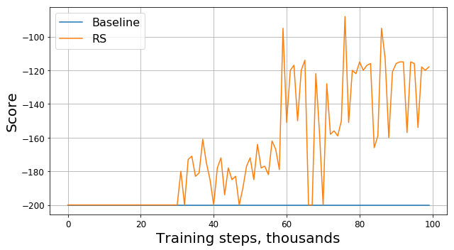
memory.push ((state, action, modified_reward, new_state, done))Now let's take a look at the new chart (it shows the original award without modifications):
Here RS is short for Reward Shaping.
Is it good to do that?
The progress is obvious: our agent obviously learned to drive up the hill, because the reward began to differ from -200. There is only one question left: if by changing the reward function, we changed the task itself, would the solution of the new problem we found be good for the old task?
To begin with, we will understand what “goodness” means in our case. Solving the problem, we are trying to find the optimal policy - one that maximizes the total reward for the episode. In this case, we can replace the word “good” with the word “optimal”, since we are looking for it. We also optimistically hope that our DQN will sooner or later find the optimal solution for the modified problem, and not get stuck in a local maximum. So, the question can be reformulated as follows: if by changing the reward function, we changed the task itself, would the optimal solution we found be optimal for the old problem?
As it turns out, we cannot provide such a guarantee in the general case. The answer depends on how we changed the function of the reward, how it was arranged earlier and how the environment itself is arranged. Fortunately, there is an article whose authors investigated how changing the reward function affects the optimality of the found solution.
First, they found a whole class of “safe” changes that are based on the potential method: where - potential, which depends only on the state. For such functions, the authors were able to prove that if the solution for the new problem is optimal, then for the old problem it is also optimal.
Second, the authors showed that for any other there is such a problem, the reward function R and the optimal solution of the modified problem, that this solution is not optimal for the original problem. This means that we cannot guarantee the goodness of the solution we found if we use a change that is not based on the method of potentials.
Thus, the use of potential functions to modify the reward function can only change the rate of convergence of the algorithm, but does not affect the final decision.
Accelerate the convergence correctly
Now that we know how to safely change the reward, we will try to modify the task again using the potential method instead of naive heuristics:
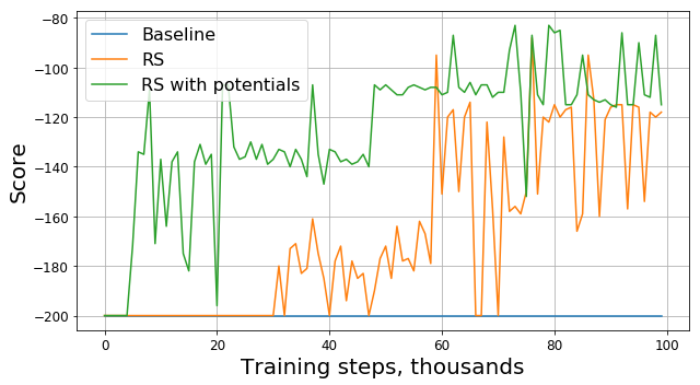
modified_reward = reward + 300 * (gamma * abs (new_state [1]) - abs (state [1]))
Look at the graph of the original award:
As it turned out, in addition to the availability of theoretical guarantees, modification of the reward with the help of potential functions also significantly improved the result, especially in the early stages. Of course, there is a possibility that it would be possible to choose more optimal hyperparameters (random seed, gamma and other coefficients) for training the agent, however, reward shaping still significantly increases the rate of convergence of the model.
Afterword
Thank you for reading to the end! I hope you enjoyed this small practice-oriented excursion to training with reinforcements. It is clear that Mountain Car is a “toy” task, however, as we could see, it can be difficult to teach an agent to solve even this seemingly simple task from a human point of view.
Source: https://habr.com/ru/post/444428/
All Articles