How error becomes sin

One urban legend says that the creator of sugar bags, sticks hanged himself, having learned that consumers do not break them in half over a cup, but carefully tear off the tip. This, of course, is not so, but if you follow this logic, then one British Guinness beer lover named William Gosset should not just hang himself, but by his rotation in the coffin already drill the Earth to the very center. And all because his landmark invention, published under the pseudonym Student , for decades used catastrophically wrong.

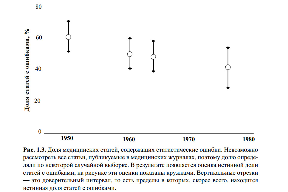
The figure above is from the book by S. Glanz. Medical and biological statistics. Per. from English - M., Praktika, 1998. - 459 p. I don’t know if anyone checked the statistical calculations for statistical errors. However, a number of modern articles on the topic, and my own experience suggest that the Student’s t-criterion remains the most famous, and therefore the most popular to use, with or without reason.

The reason for this is superficial education (strict teachers teach that it is necessary to “check statistics”, otherwise, uuuuuu!), Ease of use (tables and online calculators are available in many) and the banal reluctance to delve into what “works that way”. Most people who have used this criterion at least once in their coursework or even scientific work will say something like: "Well, we compared 5 evil schoolchildren and 7 schoolchildren-gamers in terms of aggression, we have the value according to the table comes close to p = 0.05, which means that the games are evil. Well, yes, not exactly, but with a 95% probability. " How many logical and methodological mistakes have they made?

The basics

What is the student's t-test based on? The logic is taken from the Bayes theorem, the mathematical basis from the Gauss distribution, the methodology is based on the analysis of variance:

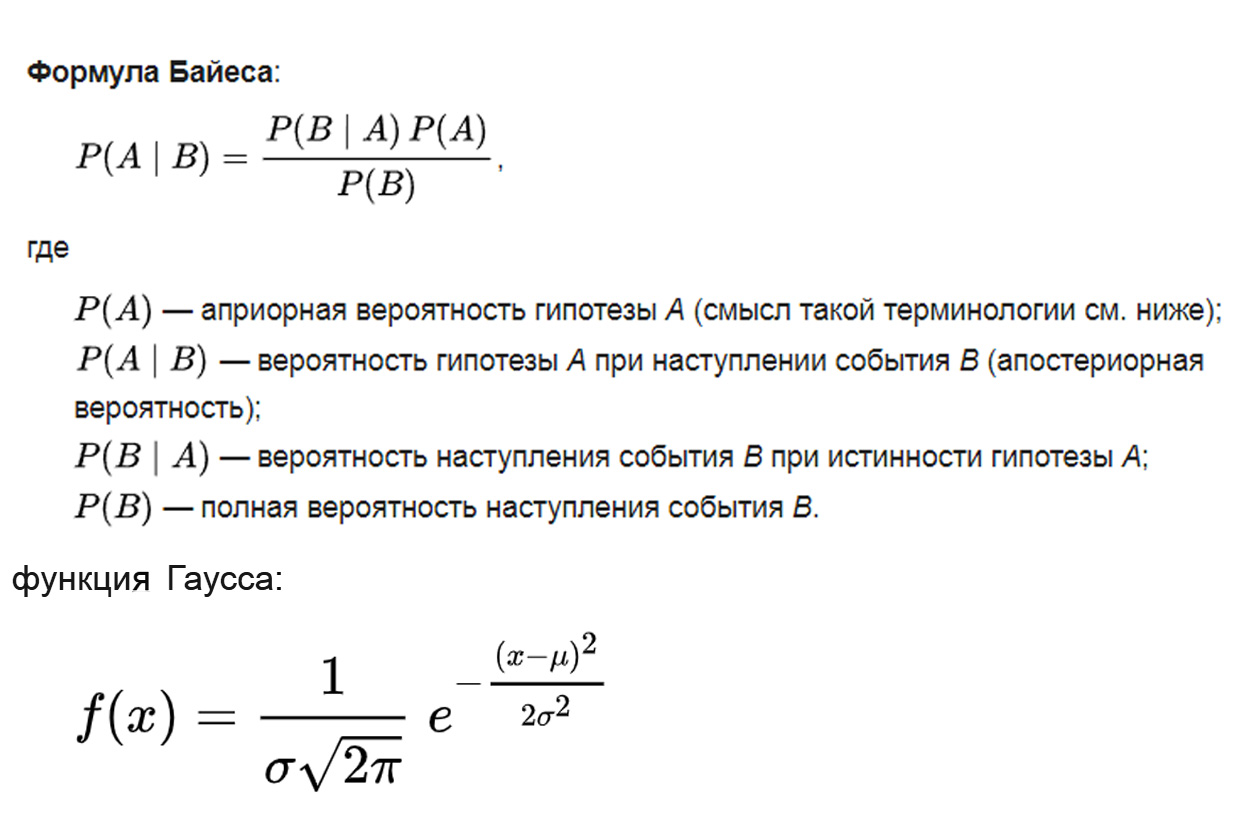
where the parameter μ is the mathematical expectation (mean) of the distribution, and the parameter σ is the standard deviation (σ ² is the variance) of the distribution.

What is analysis of variance? Imagine an audience of Habr, sorted by the number of people of each of certain ages. The number of people according to age will most likely be subject to a normal distribution - according to the Gauss function:

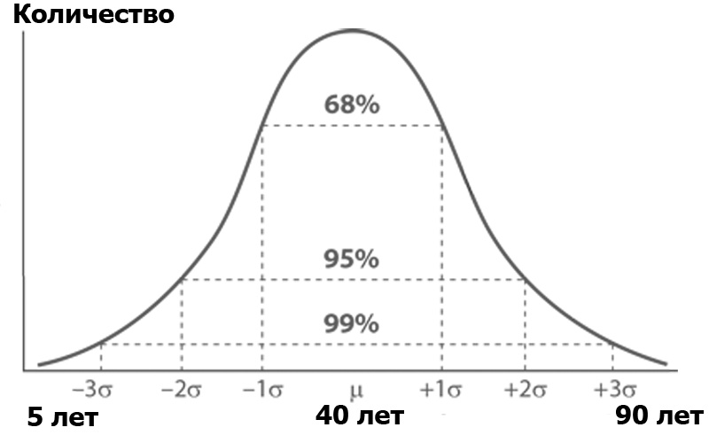
A normal distribution has an interesting property — almost all of its values ​​lie in the limit of three standard deviations from the mean. What is standard deviation? This is the root of the variance. Dispersion , in turn, is the sum of the squares of the difference of all members of the population and the average value divided by the number of these members:

$$

$$σ_ {n} ^ {2} = {\ frac {1} {n}} \ sum \ limits _ {{i = 1}} ^ {n} \ left (X_ {i} - {\ bar {X} } \ right) ^ {2}$$

That is, each value was subtracted from the average, squared to kill the minuses, and then taken the average, stupidly summing and dividing by the number of these values. The result is a measure of the average dispersion of values ​​relative to the average — dispersion.

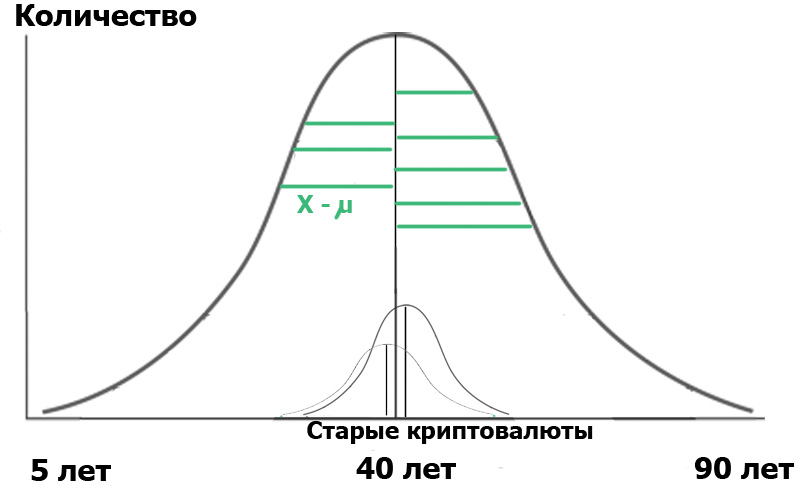
Imagine that we selected two samples in this population : readers of the Cryptocurrency hub and readers of the Old Iron hub. By making a random sample, we always get distributions close to normal . And now we have small distributors inside our population:

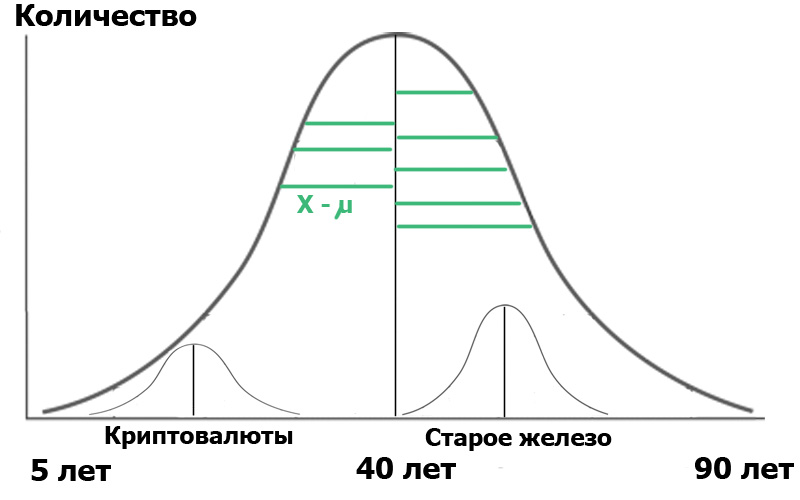
For clarity, I showed the green segments - the distance from the distribution points to the average value. If the lengths of these green segments are squared, summed and averaged, this will be the variance.

And now - attention. We can characterize the population through these two small samples. On the one hand, the sample variances characterize the variance of the entire population. On the other hand, the mean values ​​of the samples themselves are also numbers for which the variance can be calculated! So: we have the average of the sample variances and the variance of the average values ​​of the samples.

Then we can conduct analysis of variance, roughly presenting it in the form of a logical formula:

$$

$$F = {\ frac {variance \: aggregate \: by \: mean \: values ​​\: samples} {variance \: aggregate \: by \: variances \: samples}}$$

What will the above formula give us? Very simple. In statistics, everything starts with the "null hypothesis", which can be formulated as "it seemed to us", "all coincidences are random" - in meaning, and "there is no connection between the two observed events" - if strictly. So, in our case, the null hypothesis is the absence of significant differences between the age distribution of our users in the two hubs. In the case of the null hypothesis, our diagram will look something like this:

This means that both the variances of the samples and their average values ​​are very close or equal to each other, and therefore, speaking very generally, our criterion

$$

$$F = {\ frac {variance \: aggregate \: by \: mean \: values ​​\: samples} {variance \: aggregate \: by \: variances \: samples}} = 1$$

But if the variances of the samples are equal, but the habrauser's age is really very different, then the numerator (the dispersion of average values) will be large, and F will be much more than one. Then the diagram will look more like in the previous figure. And what will it give us? Nothing, if not pay attention to the wording: the null hypothesis is the absence of significant differences.

But the importance ... we ask it ourselves. It is denoted as α and has the following meaning: the level of significance is the maximum acceptable probability of mistakenly rejecting the null hypothesis . In other words, we will consider our event as a significant difference of one group from another, only if the probability P of our error is less than α. This is the notorious p <0.05, because usually in biomedical research the significance level is set at 5%.

Well, then - it's simple. Depending on α, there are critical values ​​of F, starting with which we reject the null hypothesis. They are available in the form of tables that we are used to using. This is what concerns variance analysis. And what about the student?

So said the student

A student criterion is just a special case of analysis of variance. Again, I will not overload you with formulas that are easy to googling, but will convey the essence:

$$

$$t = {\ frac {difference \: mean \: values ​​\: samples} {standard \: error \: differences \: selective \: mean}}$$

So, all this long explanation needed to be very rude and cursory, but clearly show what the t-criterion is based on. And accordingly, from which of its inherent properties directly restrict its use, on which so often even professional scientists are mistaken.

Property one: normal distribution.

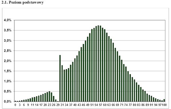
This is a couple of years as a timeline for the distribution of points for passing the Polish state exam. What can be concluded from it? What this exam does not pass only completely beaten gopnik? What do teachers "pull off" students? No, only one - for the distribution that is different from the normal one, it is impossible to apply parametric analysis criteria, such as Student's tutorial. If you have a one-sided, jagged, wavy, discrete distribution graph - forget about the t-criterion, you cannot use it. However, it is sometimes successfully ignored even by serious scientific work.

What to do in this case? Use the so-called non-parametric analysis criteria. They implement a different approach, namely, data ranking, that is, a departure from the values ​​of each of the points to the rank assigned to it. These criteria are less accurate than parametric, but at least their use is correct, in contrast to the unjustified use of the parametric criterion on an abnormal population. Of these criteria, the Mann-Whitney U-criterion is most known, and it is often used as a “for a small sample” criterion. Yes, it allows you to deal with samples up to 5 points, but this, as should be clear already, is not its main purpose.

Property two: do you remember the formula? The values ​​of the F-criterion changed with the difference (increased dispersion) of the average values ​​of the samples . But the denominator, that is, the variances themselves, should not change. Therefore, another criterion of applicability should be equality of variances. The fact that this check is observed even less often is stated, for example, here: Errors of statistical analysis of biomedical data. Leonov V.P. International Journal of Medical Practice, 2007, vol. 2, p . 19-35 .

Property Three: Comparison of two samples. They like to compare t-criterion for comparison of more than two groups. This is done, as a rule, as follows: the differences of group A from B, B from C and A from C are compared in pairs. Then, on the basis of this, a conclusion is drawn that is absolutely incorrect. In this case, the effect of multiple comparisons.
Having obtained a sufficiently high value of t in any of the three comparisons, the researchers report that “P <0.05”. But in reality, the probability of error significantly exceeds 5%.

Why?

We understand: for example, a level of significance of 5% was adopted in the study. This means that the maximum acceptable probability of mistakenly rejecting the null hypothesis when comparing groups A and B is 5%. It would seem all right? But exactly the same error will occur in the case of comparing groups B and C, and when comparing groups A and C too. Consequently, the probability of making a mistake as a whole with such an assessment will not be 5%, but much more. In general, this probability is
P ′ = 1 - (1- 0.05) ^ k
where k is the number of comparisons.

Then, in our study, the probability of making a mistake when rejecting the null hypothesis is approximately 15%. When comparing the four groups, the number of pairs and, accordingly, possible pairwise comparisons is 6. Therefore, at a significance level in each of the comparisons, 0.05
the probability of mistakenly detecting a difference in at least one is no longer 0.05, but 0.31.

This error is still easy to fix. One way is to introduce the Bonferroni amendment. Bonferroni inequality tells us that if we apply the criteria k times
with a level of significance α, then the probability in at least one case to find the difference where it does not exist does not exceed the product of k by α. From here:
α ′ <αk,
where α ′ is the probability to at least once mistakenly reveal differences. Then our problem is solved very simply: we need to divide our level of significance by the Bonferroni amendment - that is, by the multiplicity of comparisons. For the three comparisons, we need to take from the t-test tables the values ​​corresponding to α = 0.05 / 3 = 0.0167. I repeat - it is very simple, but this amendment cannot be ignored. Yes, by the way, it is also not worthwhile to get involved in this amendment, after dividing by 8 the values ​​of the t-criterion, they become unnecessarily exhausted.

Next come the "little things" that very often do not notice. I deliberately do not provide here the formulas in order not to reduce the readability of the text, but it should be remembered that the t-test calculations vary for the following cases:

• The different size of the two samples (in general, it must be remembered that in the general case we compare two groups according to the formula for the two-sample criterion);

  
  

• The presence of dependent samples. These are cases when data from one patient are measured at different time intervals, data from a group of animals before and after the experiment, etc.

  
  

Finally, for you to present the full scale of what is happening, I present more recent data on the incorrect use of the t-test. The figures are for 1998 and 2008 for a number of Chinese scientific journals, and speak for themselves. I really want this to turn out to be more of a careless design than a lack of reliable scientific data:

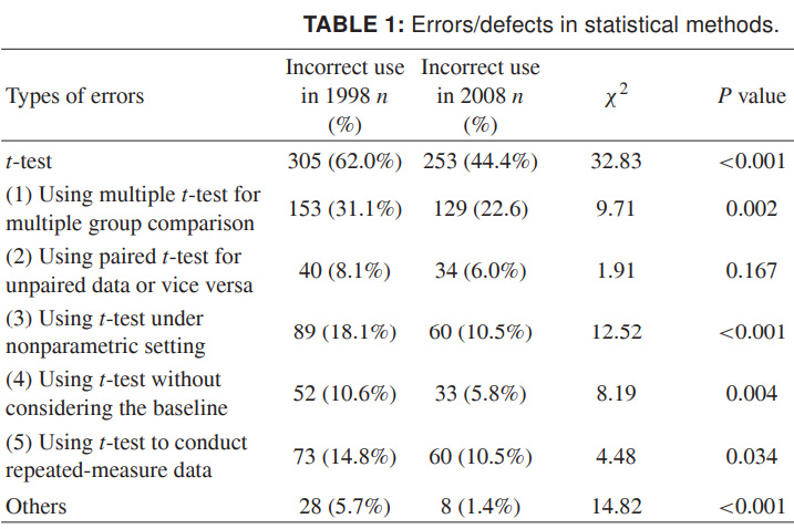
Source: Misuse of Statistical Methods in 10 Leading Chinese Medical Journals in 1998 and 2008. Shunquan Wu et al., The Scientific World Journal, 2011, 11, 2106–2114

Remember, the low significance of the results is not such a sad thing as a false result. You can not bring to scientific sin - false conclusions - the distortion of data incorrectly applied statistics.

About logical interpretation, including incorrect, statistical data, I, perhaps, I will tell separately.

Count correctly.