Understanding Q-learning, the problem of "walking on a rock"

Hi, Habr! I bring to your attention the translation of the article “Understanding Q-Learning, the Cliff Walking problem” by Lucas Vazquez .

In the last post, we presented the problem of "Walking on a rock" and stopped at a terrible algorithm that did not make sense. This time we will reveal the secrets of this gray box and see that it is not so bad at all.

Summary

We concluded that by maximizing the amount of future rewards, we also find the fastest way to the goal, so our goal now is to find a way to do it!

Introduction to Q-Learning

• Let's start by building a table that measures how well a particular action will perform in any state (we can measure it with a simple scalar value, so the larger the value, the better the action)
• This table will have one row for each state and one column for each action. In our world, the grid has 48 (4 to Y to 12 to X) states and 4 actions are allowed (up, down, left, right), so the table will be 48 x 4.
• The values ​​stored in this table are called “Q-values”.
• These are estimates of the amount of future awards. In other words, they estimate how much more rewards we can receive until the end of the game, being in state S and performing action A.
• We initialize the table with random values ​​(or some constant, for example, all zeros).

The optimal “Q-table” has values ​​that allow us to take the best actions in each state, ultimately giving us the best way to win. The problem is solved, cheers, masters of robots :).

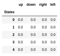
Q-values ​​of the first five states.

Q-learning

• Q-learning is an algorithm that “learns” these values.
• At every step we get more information about the world.
• This information is used to update the values ​​in the table.

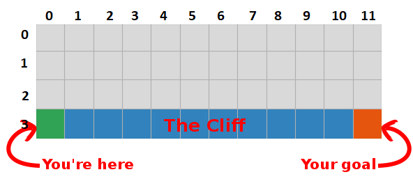
For example, suppose we are one step away from the goal (square [2, 11]), and if we decide to go down, we will receive a reward of 0 instead of -1.
We can use this information to update the value of the state-action pair in our table, and the next time we visit it, we will already know that going down gives us a reward of 0.

Now we can spread this information even further! Since we now know the path to the target from the square [2, 11], any action that leads us to the square [2, 11] will also be good, so we update the Q-value of the square that leads us to [2, 11] , to be closer to 0.

And that, ladies and gentlemen, is the essence of Q-learning!

Please note that every time we reach a goal, we increase our “map” of how to achieve the goal by one square, so after a sufficient number of iterations we will have a complete map that will show us how to get to the goal from each state.

The path is generated by taking the best actions in each state. Green tonality represents the value of a better action, more saturated tonalities represent higher values. The text represents the value for each action (up, down, right, left).
')

Bellman equation

Before we talk about code, let's talk about mathematics: the basic concept of Q-learning, the Bellman equation.

• First, let's forget γ in this equation.
• The equation states that the value of Q for a certain state-action pair must be the reward obtained when moving to a new state (by performing this action), added to the value of the best action in the next state.

In other words, we disseminate information about the values ​​of actions one step at a time!

But we can decide that receiving an award right now is more valuable than receiving an award in the future, and therefore we have γ, a number from 0 to 1 (usually from 0.9 to 0.99), which is multiplied by the award in the future, devaluing future rewards.

So, given γ = 0.9 and applying this to some states of our world (grid), we have:

We can compare these values ​​with those given above in the GIF and see that they are the same.

Implementation

Now that we have an intuitive understanding of how Q-learning works, we can start thinking about realizing all of this, and we will use the Q-learning pseudo-code from Sutton’s book as a guide.

Pseudocode from Sutton's book.

Code:

# Initialize Q arbitrarily, in this case a table full of zeros q_values = np.zeros((num_states, num_actions)) # Iterate over 500 episodes for _ in range(500): state = env.reset() done = False # While episode is not over while not done: # Choose action action = egreedy_policy(q_values, state, epsilon=0.1) # Do the action next_state, reward, done = env.step(action) # Update q_values td_target = reward + gamma * np.max(q_values[next_state]) td_error = td_target - q_values[state][action] q_values[state][action] += learning_rate * td_error # Update state state = next_state 

• First, we say: “For all states and actions, we initialize Q (s, a) arbitrarily,” which means that we can create our table of Q-values ​​with any values ​​that we like, they can be random, they can to be some kind of constant doesn't matter. We see that in row 2 we create a table full of zeros.

We also say: “The value of Q for the final states is zero”, we cannot take any actions in the final states, so we consider the value for all actions in this state to be zero.

• For each episode, we have to “initialize S”, this is just a fancy way of saying “reload the game”, in our case it means putting the player to the starting position; in our world there is a method that does just that, and we are calling it in line 6.
• For each time step (each time we need to act) we must choose an action derived from Q.

Remember, I said “we are taking actions that have the greatest value in every condition?

When we do this, we use our Q-values ​​to create a policy; in this case, it will be a greedy policy, because we always take actions that, in our opinion, are best in every state, therefore it is said that we act greedily.

Whisk

But there is a problem with this approach: imagine that we are in a maze that has two rewards, one of which is +1 and the other is +100 (and every time we find one of them, the game ends). Since we always take actions that we consider to be the best, we will be stuck with the first award found, always returning to it, therefore, if we first recognize the +1 award, we will miss the big +100 award.

Decision

We need to make sure that we have studied our world enough (this is an amazingly difficult task). This is where ε comes into play. ε in the greedy algorithm means that we have to act greedily, BUT do random actions as a percentage of ε in time, thus, with an infinite number of attempts, we must investigate all the states.

The action is chosen in accordance with this strategy in line 12, with epsilon = 0.1, which means that we are exploring the world 10% of the time. The implementation of the policy is as follows:

 def egreedy_policy(q_values, state, epsilon=0.1): # Get a random number from a uniform distribution between 0 and 1, # if the number is lower than epsilon choose a random action if np.random.random() < epsilon: return np.random.choice(4) # Else choose the action with the highest value else: return np.argmax(q_values[state]) 

In line 14 in the first listing, we call the step method to perform the action, the world returns us the next state, reward, and information about the end of the game.

Let's go back to the math:

We have a long equation, let's think about it:

If we take α = 1:

What exactly coincides with the Bellman equation, which we saw a few paragraphs ago! So we already know that this is the string responsible for disseminating information about the values ​​of the states.

But usually α (mostly known as learning speed) is much less than 1, its main goal is to avoid big changes in one update, so instead of flying to a goal, we slowly approach it. In our tabular approach, setting α = 1 does not cause any problems, but when working with neural networks (more on this in the next articles) everything can easily get out of control.

Looking at the code, we see that in line 16 in the first listing we defined td_target, this is the value we should get closer to, but instead of going directly to this value in line 17, we calculate td_error, we will use this value in conjunction with the speed learning to move slowly towards the goal.

Remember that this equation is the essence of Q-Learning.

Now we just need to update our state, and everything is ready, this is line 20. We repeat this process until we reach the end of the episode, dying in the rocks or reaching the goal.

Conclusion

Now we intuitively understand and know how to code Q-Learning (at least the tabular version), be sure to check all the code used for this post, available on GitHub .

Visualization of the learning process test:

Note that all actions begin with a value greater than its final value; this is a trick to stimulate the exploration of the world.