A guide to using pandas for analyzing large data sets.
When using the pandas library to analyze small data sets that do not exceed 100 megabytes, performance rarely becomes a problem. But when it comes to examining datasets that can reach several gigabytes in size, performance problems can lead to a significant increase in the duration of the data analysis and can even cause analysis to be impossible due to lack of memory.
While tools like Spark can efficiently handle large data sets (from hundreds of gigabytes to several terabytes), in order to fully utilize their capabilities you usually need powerful and expensive hardware. And, in comparison with pandas, they are not distinguished by a rich set of tools for quality cleaning, research and data analysis. For medium-sized datasets, it is best to try to use pandas more effectively, rather than switching to other tools.

')
In the material we are publishing today, we will talk about the peculiarities of working with memory when using pandas, and how, simply selecting the appropriate types of data stored in the columns of the
We will work with Major League baseball data collected over 130 years and taken from Retrosheet .
Initially, this data was presented in the form of 127 CSV files, but we merged them into one data set using csvkit and added, as the first row of the resulting table, a row with column names. If you want, you can download our version of this data and experiment with it by reading the article.
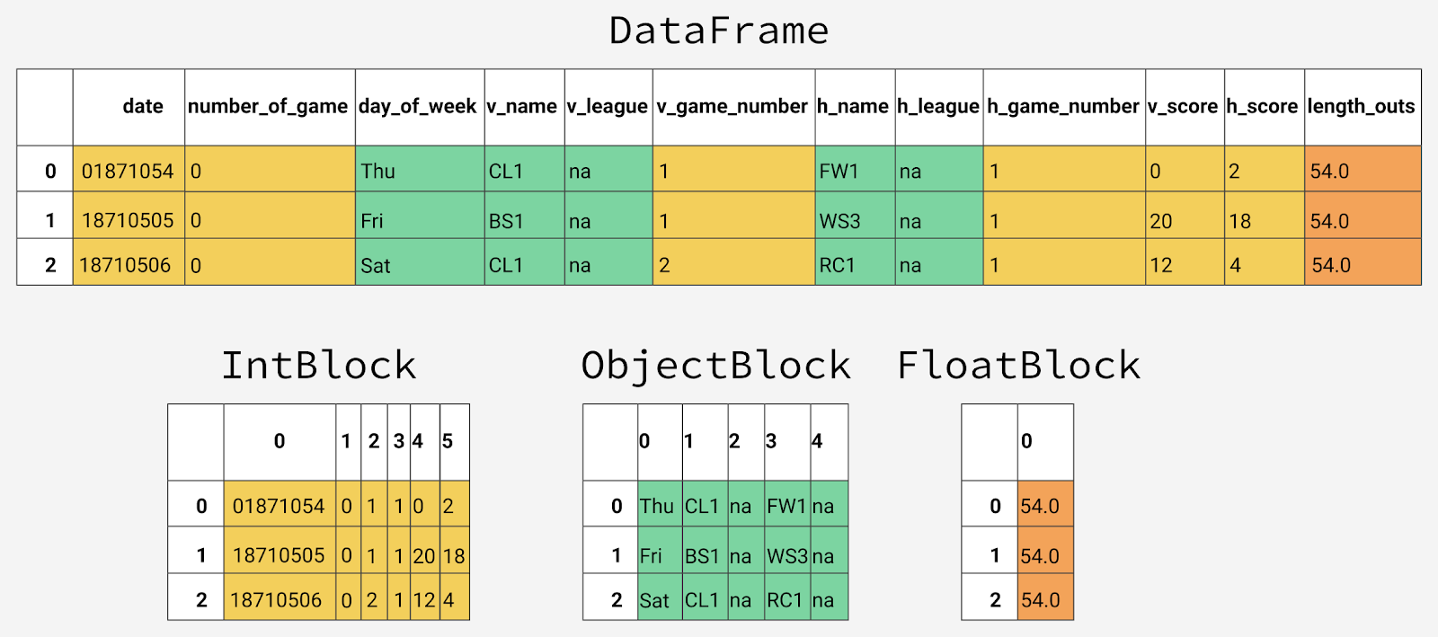
We start by importing the dataset and take a look at its first five lines. You can find them in this table, on the
Below are information about the most important columns of the table with this data. If you want to read the explanations for all columns - here you can find a dictionary of data for the entire data set.
To find out general information about the
By default, pandas, for the sake of saving time,
Here is the information we managed to get:
As it turned out, we have 171,907 rows and 161 columns. The pandas library automatically figured out the data types. There are 83 columns with numeric data and 78 columns with objects. Object columns are used to store string data, and in cases where the column contains data of different types.
Now, in order to better understand how you can optimize the memory usage of this
Inside pandas, data columns are grouped into blocks with values of the same type. Here is an example of how pandas stores the first 12 columns of a
Internal representation of data of different types in pandas
You may notice that blocks do not store information about column names. This happens because the blocks are optimized for storing values that are in the cells of the table of the
Each data type has a specialized class in the
Since data of different types is stored separately, we investigate the use of memory by different types of data. Let's start with the average memory usage for different types of data.
As a result, it appears that the average indicators of memory usage for data of different types look like this:
This information gives us to understand that most of the memory goes to 78 columns that store object values. We'll talk more about this later, but for now let's think about whether we can improve the use of memory by columns that store numeric data.
As we have said, pandas presents numeric values as
Many data types in pandas have many subtypes that can use fewer bytes to represent each value. For example, the type
A value of type
To check the minimum and maximum values suitable for storage using each integer subtype, you can use the
Having executed this code, we get the following data:
Here you can pay attention to the difference between the types of
The
Here is the result of a memory consumption study:
As a result, you can see a drop in memory usage from 7.9 to 1.5 megabytes, that is, we have reduced memory consumption by more than 80%. The overall impact of this optimization on the original
Do the same with columns containing floating point numbers.
The result is the following:
As a result, all the columns that store floating-point numbers with the
Create a copy of the original
Here's what we got:
Although we have significantly reduced memory consumption by columns storing numeric data, in general, for the entire
Before we do this optimization, let's take a closer look at how strings are stored in pandas, and compare this with how numbers are stored here.
The
This restriction leads to the fact that the lines are not stored in continuous fragments of memory, their representation in memory is fragmented. This leads to an increase in memory consumption and slowing down the speed of working with string values. Each element in the column storing an object data type is actually a pointer that contains an “address” at which the present value is located in memory.
Below is a diagram based on this material, which compares the storage of numeric data using the NumPy data types and the storage of strings using the built-in Python data types.

Storing numeric and string data
Here you can remember that above, in one of the tables, it was shown that variable memory is used to store object type data. Although each pointer occupies 1 byte of memory, each specific string value occupies the same amount of memory that would be used to store a single string in Python. To confirm this, we use the
So, first examine the usual lines:
Here the data on the use of memory look like this:
Now let's look at how the use of strings in the
Here we get the following:
You can see here that the sizes of strings stored in
Categorical variables appeared in pandas version 0.15. The corresponding type,
Baseline and categorical data using the int8 subtype
In order to understand exactly where we can use categorical data to reduce memory consumption, find out the number of unique values in the columns that store values of object types:
What we have, you can find in this table, on the sheet, the
For example, in the
Before we do full-scale optimization, let's select some single column that stores object data, at least
As already mentioned, this column contains only 7 unique values. To convert it to a categorical type, we use the
Here's what we got:
As you can see, although the column type has changed, the data stored in it looks the same as before. Let's look now at what is happening inside the program.
In the following code, we use the
We manage to figure out the following:
Here you can notice that each unique value is assigned an integer value, and that the column is now of type
Now let's compare the memory consumption before and after converting the
This is what happens:
As you can see, at first 9.84 megabytes of memory were consumed, and after optimization only 0.16 megabytes, which means 98% improvement of this indicator. Note that working with this column probably demonstrates one of the most profitable optimization scenarios, when only 7 unique values are used in a column containing approximately 172,000 items.
Although the idea of converting all columns to this data type looks attractive, before you do this, you should consider the negative side effects of such a conversion. So, the most serious disadvantage of this transformation is the impossibility of performing arithmetic operations on categorical data. This also applies to conventional arithmetic operations, and using methods like
We should limit the use of the
Create a loop that iterates through all the columns that store data of the
Now let's compare what happened after optimization with what it was before:
We get the following:
, , ,
:
. - . ,
:
:
,
:
:
, . pandas.read_csv() , . ,
, , . , .
, , .
- :
:
,
,
, , , . .

,
, 1920- , , 50 , .
, , , 50 , .
, .
, 1940- .
pandas, ,
, , , , , , pandas, , .
Dear readers! eugene_bb . - , — .

While tools like Spark can efficiently handle large data sets (from hundreds of gigabytes to several terabytes), in order to fully utilize their capabilities you usually need powerful and expensive hardware. And, in comparison with pandas, they are not distinguished by a rich set of tools for quality cleaning, research and data analysis. For medium-sized datasets, it is best to try to use pandas more effectively, rather than switching to other tools.
')
In the material we are publishing today, we will talk about the peculiarities of working with memory when using pandas, and how, simply selecting the appropriate types of data stored in the columns of the
DataFrame tabular data DataFrame , to reduce memory consumption by almost 90%.Work with data about baseball games
We will work with Major League baseball data collected over 130 years and taken from Retrosheet .
Initially, this data was presented in the form of 127 CSV files, but we merged them into one data set using csvkit and added, as the first row of the resulting table, a row with column names. If you want, you can download our version of this data and experiment with it by reading the article.
We start by importing the dataset and take a look at its first five lines. You can find them in this table, on the
import pandas as pd gl = pd.read_csv('game_logs.csv') gl.head() Below are information about the most important columns of the table with this data. If you want to read the explanations for all columns - here you can find a dictionary of data for the entire data set.
date- The date of the game.v_name- Name of the guest team.v_league- guest team league.h_name- The name of the home team.h_league- home team league.v_score- Guest team points.h_score-h_scoreteam points.v_line_score- Summary of guest team points, for example,010000(10)00.h_line_score- Summary by points of the home team, for example -010000(10)0X.park_id- ID of the field where the game was played.attendance- The number of viewers.
To find out general information about the
DataFrame object, you can use the DataFrame.info () method. Through this method, you can learn about the size of the object, the types of data and memory usage.By default, pandas, for the sake of saving time,
DataFrame rough information about the memory usage of a DataFrame object. We are interested in accurate information, so we set the memory_usage parameter to 'deep' . gl.info(memory_usage='deep') Here is the information we managed to get:
<class 'pandas.core.frame.DataFrame'> RangeIndex: 171907 entries, 0 to 171906 Columns: 161 entries, date to acquisition_info dtypes: float64(77), int64(6), object(78) memory usage: 861.6 MB As it turned out, we have 171,907 rows and 161 columns. The pandas library automatically figured out the data types. There are 83 columns with numeric data and 78 columns with objects. Object columns are used to store string data, and in cases where the column contains data of different types.
Now, in order to better understand how you can optimize the memory usage of this
DataFrame object, let's talk about how pandas stores data in memory.Internal representation of the DataFrame object
Inside pandas, data columns are grouped into blocks with values of the same type. Here is an example of how pandas stores the first 12 columns of a
DataFrame object.Internal representation of data of different types in pandas
You may notice that blocks do not store information about column names. This happens because the blocks are optimized for storing values that are in the cells of the table of the
DataFrame object. For storing information about the correspondence between the row and column indexes of a dataset and what is stored in blocks of the same type of data, is responsible the class BlockManager . It plays the role of an API that provides access to the underlying data. When we read, edit, or delete values, the DataFrame class interacts with the BlockManager class to convert our requests to calls to functions and methods.Each data type has a specialized class in the
pandas.core.internals module. For example, pandas uses the ObjectBlock class to represent blocks containing string columns, and the FloatBlock class to represent blocks containing columns that FloatBlock floating-point numbers. For blocks representing numeric values that look like integers or floating point numbers, pandas combines the columns and stores them as the ndarray data ndarray the NumPy library. This data structure is based on the array C, the values are stored in a continuous block of memory. Thanks to this data storage scheme, access to data fragments is very fast.Since data of different types is stored separately, we investigate the use of memory by different types of data. Let's start with the average memory usage for different types of data.
for dtype in ['float','int','object']: selected_dtype = gl.select_dtypes(include=[dtype]) mean_usage_b = selected_dtype.memory_usage(deep=True).mean() mean_usage_mb = mean_usage_b / 1024 ** 2 print("Average memory usage for {} columns: {:03.2f} MB".format(dtype,mean_usage_mb)) As a result, it appears that the average indicators of memory usage for data of different types look like this:
Average memory usage for float columns: 1.29 MB Average memory usage for int columns: 1.12 MB Average memory usage for object columns: 9.53 MB This information gives us to understand that most of the memory goes to 78 columns that store object values. We'll talk more about this later, but for now let's think about whether we can improve the use of memory by columns that store numeric data.
Subtypes
As we have said, pandas presents numeric values as
ndarray NumPy data structures and stores them in continuous memory blocks. This storage model allows you to save memory and quickly access values. Since pandas represents each value of the same type using the same number of bytes, and ndarray structures store information about the number of values, pandas can quickly and accurately return information about the amount of memory consumed by columns storing numerical values.Many data types in pandas have many subtypes that can use fewer bytes to represent each value. For example, the type
float has subtypes float16 , float32 and float64 . The number in the type name indicates the number of bits that the subtype uses to represent values. For example, in the subtypes just listed, 2, 4, 8, and 16 bytes are used for data storage, respectively. The following table shows the subtypes most commonly used in pandas data types.| Memory usage, bytes | Floating point number | Integer | Unsigned integer | date and time | Boolean value | An object |
| one | int8 | uint8 | bool | |||
| 2 | float16 | int16 | uint16 | |||
| four | float32 | int32 | uint32 | |||
| eight | float64 | int64 | uint64 | datetime64 | ||
| Variable memory | object |
A value of type
int8 uses 1 byte (8 bits) to store numbers and can represent 256 binary values (2 to 8 degrees). This means that this subtype can be used to store values in the range from -128 to 127 (including 0).To check the minimum and maximum values suitable for storage using each integer subtype, you can use the
numpy.iinfo() method. Consider an example: import numpy as np int_types = ["uint8", "int8", "int16"] for it in int_types: print(np.iinfo(it)) Having executed this code, we get the following data:
Machine parameters for uint8 --------------------------------------------------------------- min = 0 max = 255 --------------------------------------------------------------- Machine parameters for int8 --------------------------------------------------------------- min = -128 max = 127 --------------------------------------------------------------- Machine parameters for int16 --------------------------------------------------------------- min = -32768 max = 32767 --------------------------------------------------------------- Here you can pay attention to the difference between the types of
uint (unsigned integer) and int (signed integer). Both types have the same capacity, but, when storing only positive values in columns, unsigned types allow for more efficient use of memory.Optimize storage of numeric data using subtypes
The
pd.to_numeric() function can be used for downward conversion of numeric types. To select integer columns, use the DataFrame.select_dtypes() method, then optimize them and compare the memory usage before and after optimization. # , , # , . def mem_usage(pandas_obj): if isinstance(pandas_obj,pd.DataFrame): usage_b = pandas_obj.memory_usage(deep=True).sum() else: # , DataFrame, Series usage_b = pandas_obj.memory_usage(deep=True) usage_mb = usage_b / 1024 ** 2 # return "{:03.2f} MB".format(usage_mb) gl_int = gl.select_dtypes(include=['int']) converted_int = gl_int.apply(pd.to_numeric,downcast='unsigned') print(mem_usage(gl_int)) print(mem_usage(converted_int)) compare_ints = pd.concat([gl_int.dtypes,converted_int.dtypes],axis=1) compare_ints.columns = ['before','after'] compare_ints.apply(pd.Series.value_counts) Here is the result of a memory consumption study:
7.87 MB
1.48 MB| Before | After | |
| uint8 | NaN | 5.0 |
| uint32 | NaN | 1.0 |
| int64 | 6.0 | NaN |
As a result, you can see a drop in memory usage from 7.9 to 1.5 megabytes, that is, we have reduced memory consumption by more than 80%. The overall impact of this optimization on the original
DataFrame object, however, is not particularly strong, since there are very few integer columns.Do the same with columns containing floating point numbers.
gl_float = gl.select_dtypes(include=['float']) converted_float = gl_float.apply(pd.to_numeric,downcast='float') print(mem_usage(gl_float)) print(mem_usage(converted_float)) compare_floats = pd.concat([gl_float.dtypes,converted_float.dtypes],axis=1) compare_floats.columns = ['before','after'] compare_floats.apply(pd.Series.value_counts) The result is the following:
100.99 MB
50.49 MB| Before | After | |
| float32 | NaN | 77.0 |
| float64 | 77.0 | NaN |
As a result, all the columns that store floating-point numbers with the
float64 data type now store float32 , which gave us a 50% reduction in memory usage.Create a copy of the original
DataFrame object, use these optimized numeric columns instead of those that were originally present in it, and look at the overall memory utilization rate after optimization. optimized_gl = gl.copy() optimized_gl[converted_int.columns] = converted_int optimized_gl[converted_float.columns] = converted_float print(mem_usage(gl)) print(mem_usage(optimized_gl)) Here's what we got:
861.57 MB
804.69 MB
Although we have significantly reduced memory consumption by columns storing numeric data, in general, for the entire
DataFrame object, memory consumption has decreased by only 7%. The source of a much more serious improvement in the situation may be the optimization of the storage of object types.Before we do this optimization, let's take a closer look at how strings are stored in pandas, and compare this with how numbers are stored here.
Comparison of number and string storage mechanisms
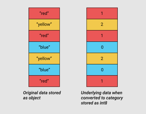
The
object type represents values using Python string objects. This is partly due to the fact that NumPy does not support the representation of missing string values. Since Python is a high-level interpreted language, it does not provide the programmer with the tools to fine-tune how data is stored in memory.This restriction leads to the fact that the lines are not stored in continuous fragments of memory, their representation in memory is fragmented. This leads to an increase in memory consumption and slowing down the speed of working with string values. Each element in the column storing an object data type is actually a pointer that contains an “address” at which the present value is located in memory.
Below is a diagram based on this material, which compares the storage of numeric data using the NumPy data types and the storage of strings using the built-in Python data types.
Storing numeric and string data
Here you can remember that above, in one of the tables, it was shown that variable memory is used to store object type data. Although each pointer occupies 1 byte of memory, each specific string value occupies the same amount of memory that would be used to store a single string in Python. To confirm this, we use the
sys.getsizeof() method. First, look at the individual lines, and then at the Series pandas object, which stores string data.So, first examine the usual lines:
from sys import getsizeof s1 = 'working out' s2 = 'memory usage for' s3 = 'strings in python is fun!' s4 = 'strings in python is fun!' for s in [s1, s2, s3, s4]: print(getsizeof(s)) Here the data on the use of memory look like this:
60
65
74
74
Now let's look at how the use of strings in the
Series object looks like: obj_series = pd.Series(['working out', 'memory usage for', 'strings in python is fun!', 'strings in python is fun!']) obj_series.apply(getsizeof) Here we get the following:
0 60 1 65 2 74 3 74 dtype: int64 You can see here that the sizes of strings stored in
Series pandas objects are similar to their sizes when working with them in Python and when presented as independent entities.Optimize data storage for object types using categorical variables
Categorical variables appeared in pandas version 0.15. The corresponding type,
category , uses in its internal mechanisms, instead of the original values stored in the columns of the table, integer values. Pandas uses a separate dictionary that matches integer and source values. This approach is useful in cases where the columns contain values from a limited set. When data stored in a column is converted into the category type, pandas uses the int subtype, which makes it possible to efficiently manage the memory and is able to represent all the unique values found in the column.Baseline and categorical data using the int8 subtype
In order to understand exactly where we can use categorical data to reduce memory consumption, find out the number of unique values in the columns that store values of object types:
gl_obj = gl.select_dtypes(include=['object']).copy() gl_obj.describe() What we have, you can find in this table, on the sheet, the
For example, in the
day_of_week column, which is the day of the week on which the game was played, there are 171907 values. Among them, only 7 unique. In general, one glance at this report is enough to understand that in many columns for representing the data of approximately 172,000 games quite a few unique values are used.Before we do full-scale optimization, let's select some single column that stores object data, at least
day_of_week , and see what happens inside the program when it is converted to a categorical type.As already mentioned, this column contains only 7 unique values. To convert it to a categorical type, we use the
.astype() method. dow = gl_obj.day_of_week print(dow.head()) dow_cat = dow.astype('category') print(dow_cat.head()) Here's what we got:
0 Thu 1 Fri 2 Sat 3 Mon 4 Tue Name: day_of_week, dtype: object 0 Thu 1 Fri 2 Sat 3 Mon 4 Tue Name: day_of_week, dtype: category Categories (7, object): [Fri, Mon, Sat, Sun, Thu, Tue, Wed] As you can see, although the column type has changed, the data stored in it looks the same as before. Let's look now at what is happening inside the program.
In the following code, we use the
Series.cat.codes attribute to find out which integer values the category type uses to represent each of the days of the week: dow_cat.head().cat.codes We manage to figure out the following:
0 4 1 0 2 2 3 1 4 5 dtype: int8 Here you can notice that each unique value is assigned an integer value, and that the column is now of type
int8 . There are no missing values, but if that were the case, the number -1 would be used to indicate such values.Now let's compare the memory consumption before and after converting the
day_of_week column to the category type. print(mem_usage(dow)) print(mem_usage(dow_cat)) This is what happens:
9.84 MB
0.16 MB
As you can see, at first 9.84 megabytes of memory were consumed, and after optimization only 0.16 megabytes, which means 98% improvement of this indicator. Note that working with this column probably demonstrates one of the most profitable optimization scenarios, when only 7 unique values are used in a column containing approximately 172,000 items.
Although the idea of converting all columns to this data type looks attractive, before you do this, you should consider the negative side effects of such a conversion. So, the most serious disadvantage of this transformation is the impossibility of performing arithmetic operations on categorical data. This also applies to conventional arithmetic operations, and using methods like
Series.min() and Series.max() without first converting the data to a real numeric type.We should limit the use of the
category type, mainly to columns that store object data, in which less than 50% of the values are unique. If all the values in a column are unique, then the use of the category type will lead to an increase in memory usage. This is due to the fact that in memory you have to store, in addition to the numeric category codes, the original string values as well. Details on category restrictions can be found in the pandas documentation .Create a loop that iterates through all the columns that store data of the
object type, finds out if the number of unique values in the columns does not exceed 50%, and if so, converts them into the category type. converted_obj = pd.DataFrame() for col in gl_obj.columns: num_unique_values = len(gl_obj[col].unique()) num_total_values = len(gl_obj[col]) if num_unique_values / num_total_values < 0.5: converted_obj.loc[:,col] = gl_obj[col].astype('category') else: converted_obj.loc[:,col] = gl_obj[col] Now let's compare what happened after optimization with what it was before:
print(mem_usage(gl_obj)) print(mem_usage(converted_obj)) compare_obj = pd.concat([gl_obj.dtypes,converted_obj.dtypes],axis=1) compare_obj.columns = ['before','after'] compare_obj.apply(pd.Series.value_counts) We get the following:
752.72 MB
51.67 MB| Before | After | |
| object | 78.0 | NaN |
| category | NaN | 78.0 |
category , , , , , , , , ., , ,
object , 752 52 , 93%. , . , , , , 891 . optimized_gl[converted_obj.columns] = converted_obj mem_usage(optimized_gl) :
'103.64 MB'. - . ,
datetime , , , . date = optimized_gl.date print(mem_usage(date)) date.head() :
0.66 MB:
0 18710504 1 18710505 2 18710506 3 18710508 4 18710509 Name: date, dtype: uint32 ,
uint32 . - datetime , 64 . datetime , , , .to_datetime() , format , YYYY-MM-DD . optimized_gl['date'] = pd.to_datetime(date,format='%Y%m%d') print(mem_usage(optimized_gl)) optimized_gl.date.head() :
104.29 MB:
0 1871-05-04 1 1871-05-05 2 1871-05-06 3 1871-05-08 4 1871-05-09 Name: date, dtype: datetime64[ns] DataFrame . , , , , , , , . , . , , , . , , DataFrame , ., . pandas.read_csv() , . ,
dtype , , , , — NumPy., , . , .
dtypes = optimized_gl.drop('date',axis=1).dtypes dtypes_col = dtypes.index dtypes_type = [i.name for i in dtypes.values] column_types = dict(zip(dtypes_col, dtypes_type)) # 161 , # 10 / # preview = first2pairs = {key:value for key,value in list(column_types.items())[:10]} import pprint pp = pp = pprint.PrettyPrinter(indent=4) pp.pprint(preview) : { 'acquisition_info': 'category', 'h_caught_stealing': 'float32', 'h_player_1_name': 'category', 'h_player_9_name': 'category', 'v_assists': 'float32', 'v_first_catcher_interference': 'float32', 'v_grounded_into_double': 'float32', 'v_player_1_id': 'category', 'v_player_3_id': 'category', 'v_player_5_id': 'category'} , , .
- :
read_and_optimized = pd.read_csv('game_logs.csv',dtype=column_types,parse_dates=['date'],infer_datetime_format=True) print(mem_usage(read_and_optimized)) read_and_optimized.head() :
104.28 MB,
,
, , , . .
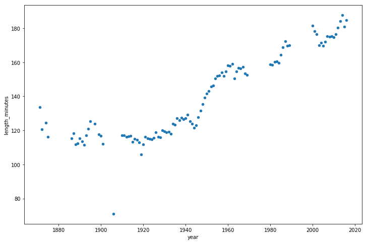
optimized_gl['year'] = optimized_gl.date.dt.year games_per_day = optimized_gl.pivot_table(index='year',columns='day_of_week',values='date',aggfunc=len) games_per_day = games_per_day.divide(games_per_day.sum(axis=1),axis=0) ax = games_per_day.plot(kind='area',stacked='true') ax.legend(loc='upper right') ax.set_ylim(0,1) plt.show() ,
, 1920- , , 50 , .
, , , 50 , .
, .
game_lengths = optimized_gl.pivot_table(index='year', values='length_minutes') game_lengths.reset_index().plot.scatter('year','length_minutes') plt.show() , 1940- .
Results
pandas, ,
DataFrame , 90%. :- , , , , .
- .
, , , , , , pandas, , .
Dear readers! eugene_bb . - , — .
Source: https://habr.com/ru/post/442516/
All Articles