LQR control system optimization

Introduction

Several articles [1,2,3] were published on Habr, directly or indirectly relating to this topic. In this regard, it is impossible not to note the publication [1] with the title “Mathematics on the fingers: linear-quadratic controller”, which popularly explains the principle of operation of the optimal LQR controller.

I wanted to continue this topic, having considered the practical application of the dynamic optimization method, but on a specific example using Python tools. First, a few words about terminology and the method of dynamic optimization.

Optimization methods are divided into static and dynamic. The control object is in a state of continuous movement under the action of various external and internal factors. Consequently, the evaluation of the control result is given during the control T, and this is the problem of dynamic optimization.

')

With the help of dynamic optimization methods, problems associated with the distribution of limited resources over a period of time are solved, and the objective function is written as an integral functional.

The mathematical apparatus for solving such problems are the variational methods: the classical calculus of variations, the maximum principle L.S. Pontryagin and R. Bellman's dynamic programming.

Analysis and synthesis of control systems is performed in the time, frequency domains and in the state space. The analysis and synthesis of control systems in the state space is introduced into the curriculum; however, the methods given in the training materials using the SQR controller are designed for the use of Matlab and do not contain practical examples of analysis.

The purpose of this publication is to examine the methods of analysis and synthesis of linear control systems in the state space using the well-known example of optimizing an electric drive and aircraft control system by means of the Python programming language.

Mathematical justification of the method of dynamic optimization

For optimization, the criteria of amplitude (MO), symmetric (CO) and compromise optima (CO) are used.

When solving optimization problems in the state space, the linear stationary system is defined by vector - matrix equations:

d o t x = f r a c d x d t = A c d o t x + B c d o t u; y = C c d o t x,

$\ dot {x} = \ frac {dx} {dt} = A \ cdot x + B \ cdot u; y = C \ cdot x,$ (one)

Integral criteria for minimum energy consumption for control and maximum performance are given by the functionals:

J_{x} = i n t_{0}^{i n f t y} (x^{T} Q x + u^{T} R u + 2 x^{T} N u) d t r i g h t a r r o w m i n,

$J_ {x} = \ int_ {0} ^ {\ infty} (x ^ {T} Qx + u ^ {T} Ru + 2x ^ {T} Nu) dt \ rightarrow min,$ (2)

J_{u} = i n t_{0}^{i n f t y} (y^{T} Q y + u^{T} R u + 2 y^{T} N u) d t r i g h t a r r o w m i n .

$J_ {u} = \ int_ {0} ^ {\ infty} (y ^ {T} Qy + u ^ {T} Ru + 2y ^ {T} Nu) dt \ rightarrow min.$ (3)

The control law u is in the form of linear feedback on state variables x or output variables y:

u = p m K x, u = p m K y

$u = \ pm Kx, u = \ pm Ky$

Such control minimizes quadratic quality criteria (2), (3). In relations (1) ÷ (3), Q and R are symmetric positive definite matrices of dimension [n × n] and [m × m], respectively; K is a matrix of constant coefficients of dimension [m × n], the values of which are not restricted. If the input parameter N is omitted, it is taken as zero.

The solution of this problem, which is called the problem of linear integral quadratic optimization (LQR optimization), in the state space is determined by the expression:

u = R^{- 1} B^{T} P x

$u = R ^ {- 1} B ^ {T} Px$

where the matrix P must satisfy the Ricatti equation:

A^{T} P + P A + P B R^{- 1} B^{T} P + Q = 0

$A ^ {T} P + PA + PBR ^ {- 1} B ^ {T} P + Q = 0$

Criteria (2), (3) are also contradictory, since the implementation of the first term requires an infinitely high power source, and for the second, an infinitely low power source. This can be explained by the following expression:

J_{x} = i n t_{0}^{i n f t y} x^{T} Q x d t

$J_ {x} = \ int_ {0} ^ {\ infty} x ^ {T} Qxdt$ ,

in which is the norm

M o d (x)

$Mod (x)$ vectors x, i.e. a measure of its oscillation in the process of regulation, and, therefore, takes smaller values in fast transients with less oscillation, and the expression:

J_{u} = i n t_{0}^{i n f t y} u^{T} R u d t

$J_ {u} = \ int_ {0} ^ {\ infty} u ^ {T} Rudt$

is a measure of the amount of energy used to control, it is a penalty for the energy costs of the system.

The constraints of the corresponding coordinates depend on the weight matrices Q, R, and N. If any element of these matrices is zero, then the corresponding coordinate has no restrictions. In practice, the choice of the values of the matrices Q, R, N is carried out by the method of expert estimates, tests, errors and depends on the experience and knowledge of the design engineer.

To solve such problems, the following MATLAB operators were used:

b e g i n b m a t r i x R, S, E e n d b m a t r i x = l q r (A, B, Q, R, N)

$\ begin {bmatrix} R, S, E \ end {bmatrix} = lqr (A, B, Q, R, N)$ and

b e g i n b m a t r i x R, S, E e n d b m a t r i x = l q r y (P_{s}, Q, R, N)

$\ begin {bmatrix} R, S, E \ end {bmatrix} = lqry (P_ {s}, Q, R, N)$ that minimize the functionals (2), (3) by the state vector x or by the output vector y.

Management Object Model

P_{s} = s s (A, B, C, D) .

$P_ {s} = ss (A, B, C, D).$ The result of the calculation is the matrix K of optimal feedbacks on state variables x, the solution of the Ricatti equation S and the eigenvalues E = eiq (A-BK) of the closed-loop control system.

Components of the functional:

J_{x} = x 0^{T} P_{1} x 0, J_{u} = x 0^{T} P_{2} x 0

$J_ {x} = x0 ^ {T} P_ {1} x0, J_ {u} = x0 ^ {T} P_ {2} x0$

where x0 is the vector of initial conditions;

P_{1}

$P_ {1}$ and

P_{2}

$P_ {2}$ - unknown matrices that are a solution of the Lyapunov matrix equations. They are found using functions;

P_{1} = l y a p (N N, Q)

$P_ {1} = lyap (NN, Q)$ and

P_{2} = l y a p (N N, K^{T} R K)

$P_ {2} = lyap (NN, K ^ {T} RK)$ ,

N N = (A + B K)^{T}

$NN = (A + BK) ^ {T}$

Features of the implementation of the dynamic optimization method of Python

Although the Python Control Systems Library [4] library has functions: control.lqr, control.lyap, however, using control.lqr is possible only if you install the slycot module, which is a problem [5]. When using the lyap function in the context of a problem, optimization leads to a control.exception.ControlArgument error: Q must be a symmetric matrix [6].

Therefore, to implement the lqr () and lyap () functions, I used scipy.linalg:

from numpy import* from scipy.linalg import* def lqr(A,B,Q,R): S =matrix(solve_continuous_are(A, B, Q, R)) K = matrix(inv(R)*(BT*S)) E= eig(AB*K)[0] return K, S, E P1=solve_lyapunov(NN,Ct*Q*C)

By the way, control should not be completely abandoned, since the functions step (), pole (), ss (), tf (), feedback (), acker (), place () and others work well.

An example of LQR optimization in the drive

(example taken from publication [7])

Consider the synthesis of a linear-quadratic controller that satisfies the criterion (2) for the control object specified in the state space by matrices:

A = \ begin {bmatrix} & -100 & 0 & 0 \\ & 143.678 & -16.667 & -195.402 \\ & 0 & 1.046 & 0 \ end {bmatrix}; B = \ begin {bmatrix} 2300 \\ 0 \\ 0 \\\ end {bmatrix}; C = \ begin {bmatrix} 1 & 0 & 0 \\ 0 & 1 & 0 \\ 0 & 0 & 1 \ end {bmatrix}; D = 0

$A = \ begin {bmatrix} & -100 & 0 & 0 \\ & 143.678 & -16.667 & -195.402 \\ & 0 & 1.046 & 0 \ end {bmatrix}; B = \ begin {bmatrix} 2300 \\ 0 \\ 0 \\\ end {bmatrix}; C = \ begin {bmatrix} 1 & 0 & 0 \\ 0 & 1 & 0 \\ 0 & 0 & 1 \ end {bmatrix}; D = 0$

As state variables are considered:

x_{1}

$x_ {1}$ - converter voltage, V;

x_{2}

$x_ {2}$ - motor current, A;

x_{3}

$x_ {3}$ - angular velocity,

c^{- 1}

$c ^ {- 1}$ . This system TP - DPT with HB: engine P nom = 30 kW; Unom = 220 V; Inom = 147 A ;;

o m e g a ω

$\ omega ω$ 0 = 169

c^{- 1}

$c ^ {- 1}$ ;

o m e g a ω

$\ omega ω$ max = 187

c^{- 1}

$c ^ {- 1}$ ; nominal moment of resistance Mn = 150 N * m; frequency of starting current = 2; thyristor converter: Unom = 230 V; Uy = 10 B; In = 300 A; the multiplicity of short-term current overload = 1,2.

When solving the problem, we take the matrix Q diagonal. As a result of the simulation, it was found that the minimum values of the matrix elements R = 84, and

Q = [[0.01, 0, 0], [0, 0.01, 0], [0, 0, 0.01]] .

$Q = [[0.01,0,0], [0, 0.01,0], [0,0,0.01]].$ In this case, there is a monotonous transition process of the angular velocity of the engine (Fig. 1). At R = 840

Q = [[0.01, 0, 0], [0, 0.01, 0], [0, 0, 0.01]]

$Q = [[0.01,0,0], [0, 0.01,0], [0,0,0.01]]$ the transition process (Fig. 2) meets the criterion of MO. The calculation of the matrices P1 and P2 is performed at x0 = [220 147 162].

Listing of the program (Fig. 1).

 # -*- coding: utf8 -*- from numpy import* from control.matlab import * from matplotlib import pyplot as plt from scipy.linalg import* def lqr(A,B,Q,R): S =matrix(solve_continuous_are(A, B, Q, R)) K = matrix(inv(R)*(BT*S)) E= eig(AB*K)[0] return K, S, E #   A=matrix([[-100,0,0],[143.678, -16.667,-195.402],[0,1.046,0]]); B=matrix([[2300], [0], [0]]); C=eye(3) D=zeros([3,1]) #    R=[[84]] Q=matrix([[0.01, 0, 0],[0, 0.01, 0],[0, 0, 0.01]]); #  LQR-  [K,S,E]=lqr(A,B,Q,R) #    N=AB*K; NN=NT; w=ss(N,B,C,D) x0=matrix([[220], [147], [162]]); Ct=CT; P1=solve_lyapunov(NN,Ct*Q*C) Kt=KT; x0t=x0.T; Jx=abs((x0t*P1*x0)[0,0]) P2=solve_lyapunov(NN,Kt*R*K); Ju=abs((x0t*P2*x0)[0,0]) fig = plt.figure() plt.suptitle('      R = %s,\n\ $J_{x}$= %s; $J_{u}$ = %s,Q=[[0.01,0,0],[0, 0.01,0],[0,0,0.01]]'%(R[0][0],round(Jx,1),round(Ju,1))) ax1 = fig.add_subplot(311) y,x=step(w[0,0]) ax1.plot(x,y,"b") plt.ylabel('$x_{1}$,B') ax1.grid(True) ax2 = fig.add_subplot(312) y,x=step(w[1,0]) ax2.plot(x,y,"b") plt.ylabel('$x_{2}$,A') ax2.grid(True) ax3 = fig.add_subplot(313) y,x=step(w[2,0]) ax3.plot(x,y,"b") plt.ylabel('$x_{3}$,$C^{-1}$') ax3.grid(True) plt.xlabel(', .') plt.show()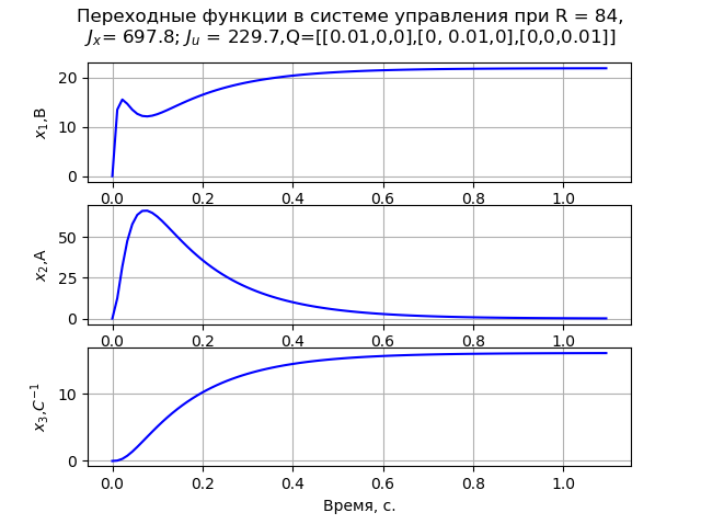

Fig. one

Program listing (Fig.2).

 # -*- coding: utf8 -*- from numpy import* from control.matlab import * from matplotlib import pyplot as plt from scipy.linalg import* def lqr(A,B,Q,R): S =matrix(solve_continuous_are(A, B, Q, R)) K = matrix(inv(R)*(BT*S)) E= eig(AB*K)[0] return K, S, E #   A=matrix([[-100,0,0],[143.678, -16.667,-195.402],[0,1.046,0]]); B=matrix([[2300], [0], [0]]); C=eye(3) D=zeros([3,1]) #    R=[[840]] Q=matrix([[0.01, 0, 0],[0, 0.01, 0],[0, 0, 0.01]]); #  LQR-  [K,S,E]=lqr(A,B,Q,R) #    N=AB*K; NN=NT; w=ss(N,B,C,D) x0=matrix([[220], [147], [162]]); Ct=CT; P1=solve_lyapunov(NN,Ct*Q*C) Kt=KT; x0t=x0.T; Jx=abs((x0t*P1*x0)[0,0]) P2=solve_lyapunov(NN,Kt*R*K); Ju=abs((x0t*P2*x0)[0,0]) fig = plt.figure() plt.suptitle('      R = %s,\n\ $J_{x}$= %s; $J_{u}$ = %s,Q=[[0.01,0,0],[0, 0.01,0],[0,0,0.01]]'%(R[0][0],round(Jx,1),round(Ju,1))) ax1 = fig.add_subplot(311) y,x=step(w[0,0]) ax1.plot(x,y,"b") plt.ylabel('$x_{1}$,B') ax1.grid(True) ax2 = fig.add_subplot(312) y,x=step(w[1,0]) ax2.plot(x,y,"b") plt.ylabel('$x_{2}$,A') ax2.grid(True) ax3 = fig.add_subplot(313) y,x=step(w[2,0]) ax3.plot(x,y,"b") plt.ylabel('$x_{3}$,$C^{-1}$') ax3.grid(True) plt.xlabel(', .') plt.show()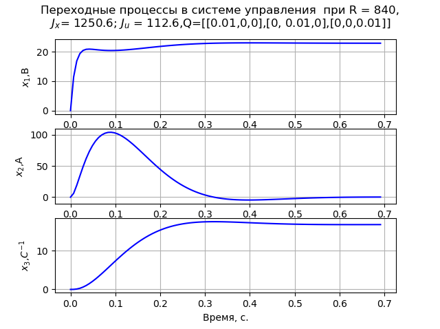

Fig. 2

By appropriate selection of the matrices R and Q, it is possible to reduce the starting current of the motor to permissible values equal to (2–2.5) In (Fig. 3). For example, when R = 840 and

Q = ([[0.01,0,0], [0,0.88,0], [0,0,0.01]] its value is 292 A, and the transition time under these conditions is 1.57 seconds.

Program listing (Fig.3).

 # -*- coding: utf8 -*- from numpy import* from control.matlab import * from matplotlib import pyplot as plt from scipy.linalg import* def lqr(A,B,Q,R): S =matrix(solve_continuous_are(A, B, Q, R)) K = matrix(inv(R)*(BT*S)) E= eig(AB*K)[0] return K, S, E #   A=matrix([[-100,0,0],[143.678, -16.667,-195.402],[0,1.046,0]]); B=matrix([[2300], [0], [0]]); C=eye(3) D=zeros([3,1]) #    R=[[840]] Q=matrix([[0.01,0,0],[0,0.88,0],[0,0,0.01]]); #  LQR-  [K,S,E]=lqr(A,B,Q,R) #    N=AB*K; NN=NT; w=ss(N,B,C,D) x0=matrix([[220], [147], [162]]); Ct=CT; P1=solve_lyapunov(NN,Ct*Q*C) Kt=KT; x0t=x0.T; Jx=abs((x0t*P1*x0)[0,0]) P2=solve_lyapunov(NN,Kt*R*K); Ju=abs((x0t*P2*x0)[0,0]) fig = plt.figure() plt.suptitle('      R = %s,\n\ $J_{x}$= %s; $J_{u}$ = %s,Q=[[0.01,0,0],[0,0.88,0],[0,0,0.01]]'%(R[0][0],round(Jx,1),round(Ju,1))) ax1 = fig.add_subplot(311) y,x=step(w[0,0]) ax1.plot(x,y,"b") plt.ylabel('$x_{1}$,B') ax1.grid(True) ax2 = fig.add_subplot(312) y,x=step(w[1,0]) ax2.plot(x,y,"b") plt.ylabel('$x_{2}$,A') ax2.grid(True) ax3 = fig.add_subplot(313) y,x=step(w[2,0]) ax3.plot(x,y,"b") plt.ylabel('$x_{3}$,$C^{-1}$') ax3.grid(True) plt.xlabel(', .') plt.show()

Pic.3

In all the considered cases, the feedbacks on voltage and current are negative, and on speed - positive, which is undesirable in terms of stability requirements. In addition, the synthesized system is astatic on the instructions and static on the load. Therefore, we consider the synthesis of a PI controller in the state space with an additional state variable

x_{4}

$x_ {4}$ - the transfer coefficient of the integrator.

The initial information is presented in the form of matrices:

A = \ begin {bmatrix} & -100 & 0 & 0 & 0 \\ & 143.678 & -16.667 & -195.402 & 0 \\ & 0 & 1.046 & 0 & 0 \\ & 0 & 0 & 1 & 0 \ end {bmatrix}; B = \ begin {bmatrix} 2300 \\ 0 \\ 0 \\ 0 \\\ end {bmatrix}; C = eye (4); D = 0

$A = \ begin {bmatrix} & -100 & 0 & 0 & 0 \\ & 143.678 & -16.667 & -195.402 & 0 \\ & 0 & 1.046 & 0 & 0 \\ & 0 & 0 & 1 & 0 \ end {bmatrix}; B = \ begin {bmatrix} 2300 \\ 0 \\ 0 \\ 0 \\\ end {bmatrix}; C = eye (4); D = 0$

Transients according to the task, corresponding to the criterion of MO, are obtained at R = 100, q11 = q22 = q33 = 0.001 and q44 = 200. Figure 4 shows transient processes of state variables, confirming the system astatism according to the task and according to the load.

Program listing (Fig.4).

 # -*- coding: utf8 -*- from numpy import* from control.matlab import * from matplotlib import pyplot as plt from scipy.linalg import* def lqr(A,B,Q,R): S =matrix(solve_continuous_are(A, B, Q, R)) K = matrix(inv(R)*(BT*S)) E= eig(AB*K)[0] return K, S, E #   A=matrix([[-100,0,0,0],[143.678, -16.667,-195.402,0],[0,1.046,0,0] ,[0,0,1,0]]); B=matrix([[2300], [0], [0],[0]]); C=matrix([[1, 0, 0,0],[0, 1, 0,0],[0, 0, 1,0],[0, 0, 0,1]]); D=matrix([[0],[0],[0],[0]]); #    R=[[100]]; Q=matrix([[0.001, 0, 0,0],[0, 0.001, 0,0],[0, 0, 0.01,0],[0, 0,0,200]]); #  LQR-  (K,S,E)=lqr(A,B,Q,R) #    N=AB*K; NN=NT; w=ss(N,B,C,D) x0=matrix([[220], [147], [162],[0]]); Ct=CT; P1=solve_lyapunov(NN,Ct*Q*C) Kt=KT; x0t=x0.T; Jx=abs((x0t*P1*x0)[0,0]) P2=solve_lyapunov(NN,Kt*R*K); Ju=abs((x0t*P2*x0)[0,0]) fig = plt.figure(num=None, figsize=(9, 7), dpi=120, facecolor='w', edgecolor='k') plt.suptitle('      LQR -',size=14) ax1 = fig.add_subplot(411) y,x=step(w[0,0]) ax1.plot(x,y,"b") plt.ylabel('out(1)') ax1.grid(True) ax2 = fig.add_subplot(412) y,x=step(w[1,0]) ax2.plot(x,y,"b") plt.ylabel('out(2)') ax2.grid(True) ax3 = fig.add_subplot(413) y,x=step(w[2,0]) ax3.plot(x,y,"b") plt.ylabel('out(3)') ax3.grid(True) ax4 = fig.add_subplot(414) y,x=step(w[3,0]) ax4.plot(x,y,"b") plt.ylabel('out(4)') ax4.grid(True) plt.xlabel(', .') plt.show()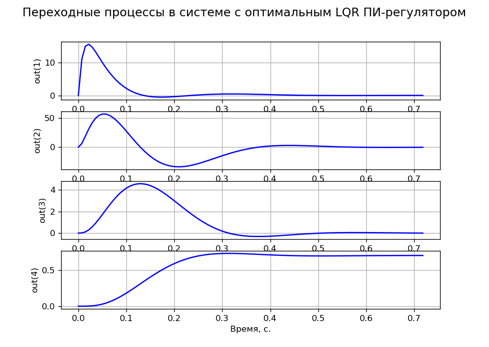

Fig. four

To determine the matrix K in the Python Control Systems Library library there are two functions K = acker (A, B, s) and K = place (A, B, s), where s is the vector - the string of the desired poles of the transfer function of the closed control system. The first command can be used only for systems with a single input on u with n≤5. The second one does not have such limitations, however the multiplicity of poles should not exceed the rank of the matrix B. An example of using the acker () operator is given in the listing and in (Fig. 5).

Program listing (Fig.5).

 # -*- coding: utf8 -*- from numpy import* from control.matlab import * from matplotlib import pyplot as plt i=(-1)**0.5 A=matrix([[-100,0,0],[143.678, -16.667,-195.402],[0,1.046,0]]); B=matrix([[2300], [0], [0]]); C=eye(3) D=zeros([3,1]) p=[[-9.71+14.97*i -9.71-14.97*i -15.39 -99.72]]; k=acker(A,B,p) H=AB*k; Wss=ss(H,B,C,D); step(Wss) w=tf(Wss) fig = plt.figure() plt.suptitle('   acker()') ax1 = fig.add_subplot(311) y,x=step(w[0,0]) ax1.plot(x,y,"b") ax1.grid(True) ax2 = fig.add_subplot(312) y,x=step(w[1,0]) ax2.plot(x,y,"b") ax2.grid(True) ax3 = fig.add_subplot(313) y,x=step(w[2,0]) ax3.plot(x,y,"b") ax3.grid(True) plt.xlabel(', .') plt.show()

Fig. five

Conclusion

The implementation of LQR optimization of the electric drive given in the publication, taking into account the use of the new lqr () and lyap () functions, will make it possible to abandon the use of the licensed program MATLAB when studying the relevant section of control theory.

An example of LQR optimization in the aircraft (LA)

(The example is taken from the publication Astrom and Mruray, Chapter 5 [8] and refined by the author of the article in terms of replacing the function lqr () and bringing the terminology to the generally accepted one)

The theoretical part, a brief theory, LQR optimization has already been discussed above, so let's move on to analyzing the code with the appropriate comments:

Required libraries and LQR controller function.

 from scipy.linalg import* # scipy   lqr from numpy import * # numpy    from matplotlib.pyplot import * #     from control.matlab import * #  control..ss()  control..step() #     lqr() m = 4; #    . J = 0.0475; #        ***2 #́-       #  . r = 0.25; #     . g = 9.8; #     /**2 c = 0.05; #   () def lqr(A,B,Q,R): X =matrix(solve_continuous_are(A, B, Q, R)) K = matrix(inv(R)*(BT*X)) E= eig(AB*K)[0] return X, K, E

Initial conditions and basic matrices of A, B, C, D models.

 xe = [0, 0, 0, 0, 0, 0];#   x   () ue = [0, m*g]; #   #   A = matrix( [[ 0, 0, 0, 1, 0, 0], [ 0, 0, 0, 0, 1, 0], [ 0, 0, 0, 0, 0, 1], [ 0, 0, (-ue[0]*sin(xe[2]) - ue[1]*cos(xe[2]))/m, -c/m, 0, 0], [ 0, 0, (ue[0]*cos(xe[2]) - ue[1]*sin(xe[2]))/m, 0, -c/m, 0], [ 0, 0, 0, 0, 0, 0 ]]) #   B = matrix( [[0, 0], [0, 0], [0, 0], [cos(xe[2])/m, -sin(xe[2])/m], [sin(xe[2])/m, cos(xe[2])/m], [r/J, 0]]) #   C = matrix([[1, 0, 0, 0, 0, 0], [0, 1, 0, 0, 0, 0]]) D = matrix([[0, 0], [0, 0]])

We build entrances and exits corresponding to incremental changes in the xy position. Vectors xd and yd correspond to the desired steady states in the system. Matrices Cx and Cy are the corresponding outputs of the model. To describe the dynamics of the system, we use the system of vector - matrix equations:

\ left \ {\ begin {matrix} xdot = Ax + Bu => xdot = (A-BK) x + xd \\ u = -K (x-xd) \\ y = Cx \\ \ end {matrix} \ right.

$\ left \ {\ begin {matrix} xdot = Ax + Bu => xdot = (A-BK) x + xd \\ u = -K (x-xd) \\ y = Cx \\ \ end {matrix} \ right.$

The dynamics of a closed loop can be modeled using the step () function, for K \ cdot xd and K \ cdot xd as input vectors, where:

 xd = matrix([[1], [0], [0], [0], [0], [0]]); yd = matrix([[0], [1], [0], [0], [0], [0]]);

The current library control 0.8.1 supports only a part of the SISO Matlab functions for creating feedback controllers, therefore for reading data from the controller, it is therefore necessary to create index vectors lat (), alt () for side-x and vertical - y dynamics.

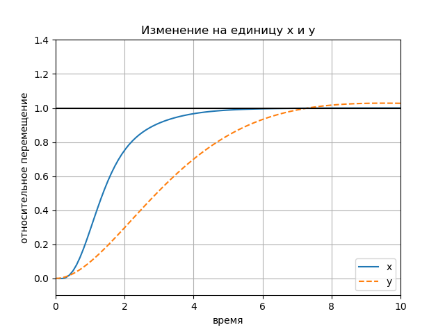
 lat = (0,2,3,5); alt = (1,4); #    Ax = (A[lat, :])[:, lat]; Bx = B[lat, 0]; Cx = C[0, lat]; Dx = D[0, 0]; Ay = (A[alt, :])[:, alt]; By = B[alt, 1]; Cy = C[1, alt]; Dy = D[1, 1]; #      K Qx1 = diag([1, 1, 1, 1, 1, 1]); Qu1a = diag([1, 1]); X,K,E =lqr(A, B, Qx1, Qu1a) K1a = matrix(K); #      x H1ax = ss(Ax - Bx*K1a[0,lat], Bx*K1a[0,lat]*xd[lat,:], Cx, Dx); (Yx, Tx) = step(H1ax, T=linspace(0,10,100)); #     y H1ay = ss(Ay - By*K1a[1,alt], By*K1a[1,alt]*yd[alt,:], Cy, Dy); (Yy, Ty) = step(H1ay, T=linspace(0,10,100));

Displays graphs one by one for each job.

 figure(); title("   x  y") plot(Tx.T, Yx.T, '-', Ty.T, Yy.T, '--'); plot([0, 10], [1, 1], 'k-'); axis([0, 10, -0.1, 1.4]); ylabel(' '); xlabel(''); legend(('x', 'y'), loc='lower right'); grid() show()

Schedule:

The influence of the amplitude of the input effects

 #     Qu1a = diag([1, 1]); X,K,E =lqr(A, B, Qx1, Qu1a) K1a = matrix(K); H1ax = ss(Ax - Bx*K1a[0,lat], Bx*K1a[0,lat]*xd[lat,:], Cx, Dx); Qu1b = (40**2)*diag([1, 1]); X,K,E =lqr(A, B, Qx1, Qu1b) K1b = matrix(K); H1bx = ss(Ax - Bx*K1b[0,lat], Bx*K1b[0,lat]*xd[lat,:],Cx, Dx); Qu1c = (200**2)*diag([1, 1]); X,K,E =lqr(A, B, Qx1, Qu1c) K1c = matrix(K); H1cx = ss(Ax - Bx*K1c[0,lat], Bx*K1c[0,lat]*xd[lat,:],Cx, Dx); figure(); [Y1, T1] = step(H1ax, T=linspace(0,10,100)); [Y2, T2] = step(H1bx, T=linspace(0,10,100)); [Y3, T3] = step(H1cx, T=linspace(0,10,100)); plot(T1.T, Y1.T, 'r-'); plot(T2.T, Y2.T, 'b-'); plot(T3.T, Y3.T, 'g-'); plot([0 ,10], [1, 1], 'k-'); axis([0, 10, -0.1, 1.4]); title("   ") legend(('1', '$1,6\cdot 10^{3}$','$4\cdot 10^{4}$'), loc='lower right'); text(5.3, 0.4, 'rho'); ylabel(' '); xlabel(''); grid() show()

Schedule:

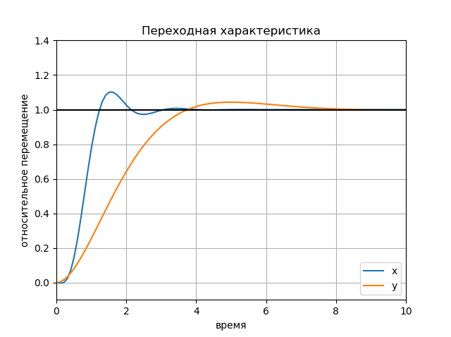
Transient response

 #  Qx    Qx2 = CT * C; Qu2 = 0.1 * diag([1, 1]); X,K,E =lqr(A, B, Qx2, Qu2) K2 = matrix(K); H2x = ss(Ax - Bx*K2[0,lat], Bx*K2[0,lat]*xd[lat,:], Cx, Dx); H2y = ss(Ay - By*K2[1,alt], By*K2[1,alt]*yd[alt,:], Cy, Dy); figure(); [Y2x, T2x] = step(H2x, T=linspace(0,10,100)); [Y2y, T2y] = step(H2y, T=linspace(0,10,100)); plot(T2x.T, Y2x.T, T2y.T, Y2y.T) plot([0, 10], [1, 1], 'k-'); axis([0, 10, -0.1, 1.4]); title(" ") ylabel(' '); xlabel(''); legend(('x', 'y'), loc='lower right'); grid() show()

Schedule:

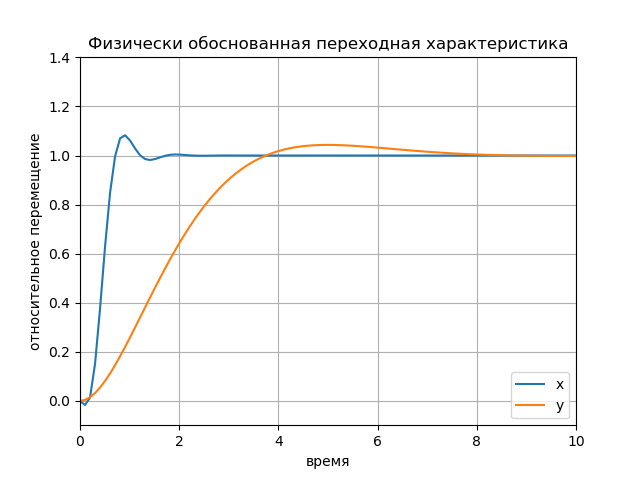
Physically sound transient response

 #    #       #   1 .     10 . Qx3 = diag([100, 10, 2*pi/5, 0, 0, 0]); Qu3 = 0.1 * diag([1, 10]); X,K,E =lqr(A, B, Qx3, Qu3) K3 = matrix(K); H3x = ss(Ax - Bx*K3[0,lat], Bx*K3[0,lat]*xd[lat,:], Cx, Dx); H3y = ss(Ay - By*K3[1,alt], By*K3[1,alt]*yd[alt,:], Cy, Dy); figure(); [Y3x, T3x] = step(H3x, T=linspace(0,10,100)); [Y3y, T3y] = step(H3y, T=linspace(0,10,100)); plot(T3x.T, Y3x.T, T3y.T, Y3y.T) axis([0, 10, -0.1, 1.4]); title("   ") ylabel(' '); xlabel(''); legend(('x', 'y'), loc='lower right'); grid() show()

Schedule:

Conclusion:

The implementation of LQR optimization in LA given in the publication taking into account the use of the new lqr () function will make it possible to abandon the use of the MATLAB licensed program when studying the relevant section of control theory.

Links

1. Mathematics on the fingers: linear-quadratic regulator.

2. State space in problems of designing optimal control systems.

3. Using the Python Control Systems Library for designing automatic control systems.

4. Python Control Systems Library.

5. Python - can not import the slycot module into spyder (RuntimeError & ImportError).

6. Python Control Systems Library.

7. Criteria for optimal control and lqr optimization in the electric drive.

Source: https://habr.com/ru/post/441582/

All Articles

LQR control system optimization

Introduction

Mathematical justification of the method of dynamic optimization

Features of the implementation of the dynamic optimization method of Python

An example of LQR optimization in the drive

Conclusion

An example of LQR optimization in the aircraft (LA)

Conclusion:

Links

More articles: