Metal search and ... neural network
The principle of operation of the pulse metal detector
One of the most popular options for the design of devices for metal search is a pulse ( pulse induction ( PI )) metal detector — an unpretentious and reliable apparatus (good detection depth, resistance to increased ground mineralization, ability to work in salt water), having various applications from military (traditional users of "impulse") before searching for gold (this hobby is particularly popular in Australia).
But he also has a significant drawback - great difficulties with discrimination, i.e. determining the type of target, for example, to find out - is it made of ferrous metal or black, or is it possible to distinguish an anti-personnel mine in a plastic case from a handful of metal debris? What is the cause of this problem?
Consider the principle of operation of a pulse metal detector.
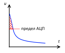
The electronic key (usually a MOSFET that can withstand a voltage of several hundred volts — for example, the popular IRF740 is used in this creation by Malaysian engineers, and in this project, based on the programmable analog-digital matrix GreenPAK , the search coil is connected to a power source (battery battery). When a control pulse is applied to the gate of the transistor (usually with a frequency of several tens or hundreds of hertz), the MOSFET opens - the circuit is closed, and a growing (gradually due to the transient process) current flows through the coil. We are waiting for a few tens or hundreds of microseconds of current rise to the desired level and ... breaking the circuit - the control impulse is over. Current through the coil and, accordingly, the magnetic flux the coil decreases sharply (to speed up the process of closing the MOSFET, the control impulse is not supplied directly to the gate, but through a special driver), which, due to the phenomenon of electromagnetic induction, causes the appearance of EMF of self-induction and a sharp increase in voltage on the coil. Then the voltage level on the coil starts to decrease. But if a conducting object (“target”) is located near the coil, then the magnetic flux through the coil decreasing with the current induces eddy currents in this target. These eddy currents create their own magnetic flux. who is trying to maintain the damped magnetic field of the coil. This effect leads to an increase in the voltage decay time at the coil, which is an indicator of the absence or presence of the target (the decision is made either by integrating the signal and estimating the integral value ( a ) or based on the signal values at several points ( b )):

Note : the pulses can be bipolar (for example, the Vallon VMH2 metal detector is a classic device used in demining):

( source )
The average value (constant component) of the magnetic field created by the metal detector is close to zero, which should (as cautiously written in the catalogs, “according to the manufacturer”) prevent undermining when searching for mines reacting to the magnetic field (although, as stated in "Metal detector handbook for humanitarian demining" , with humanitarian demining such an incident is unlikely).
Along with the described variant with one coil, combining the functions of transmitting and receiving, there are pulsed metal detectors with two separate coils. This scheme is applied not only in the field of metal search, but also in flaw detection ( Pulsed Eddy Current (PEC) Testing ) - link 1 , link 2 . In this case, one of the coils ( transmit / drive coil ) serves to excite eddy currents in the target, and the other ( receive / pickup coil ) serves as a magnetic field sensor. This approach makes it possible to analyze the magnetic field not only at the stage of decreasing (after disconnecting the power source from the transmitting coil), but also at the increasing stage (after connecting the power supply to the transmitting coil):

Here is a great description of this technology:
Discrimination issue
The problem of recognition of the type of metal arises from the fact that the resulting voltage curve on the coil is influenced by the size and shape of the target, its distance from the coil and electrical (conductivity ) and magnetic (magnetic permeability ) properties of the target material.
Here are a few quotes on this topic:
(source: Ahmet S. Turk, Koksal A. Hocaoglu, Alexey A. Vertiy Subsurface Sensing)
')
One approach to solving this problem is to use Double-D ( DD ) coils instead of the usual monoloop, for example, in popular Minelab GPX series metal detectors:

( source )
In such a coil, the transmitting ( TX ) and receiving ( RX ) windings are separated:
( source )
In this case, the signal from the target is analyzed not only when decreasing, but also when the current increases in the transmitting coil. But this discrimination is not very reliable:

( source )
But what about the single-loop reel? In many works ( reference 1 reference 2 reference 3 ) it is indicated that the signal in the coil from the target can be represented as a weighted sum of damped exponential signals whose maximum values and time constants are individual and depend on the material, size and shape of the target:
In the work " Discrimination experiments with the US Army's standard metal detector, " it is reported that in experiments conducted by the authors of the article, small objects were well characterized by one exhibitor , and for large objects, two were needed - .
This article indicates that the time constant of the exponential component can be represented as the ratio of equivalent inductance and resistance and gives its expression for a cylinder with a base radius and tall :
This paper presents the expression of the decay time constant of eddy currents for a sphere of radius :
,
Where - the result of solving the equation
Note : such analytical expressions can be obtained only for simple symmetric bodies. Therefore, to study the eddy currents, you can use software packages for numerical simulation of electromagnetic processes. As an example, the simulation of electromagnetic brakes on eddy currents in the COMSOL Multiphysics package:
( source )
As you can see, the expressions for the time constant together include the magnetic permeability, electrical conductivity and the size of the target. It is not so simple to single out the influence of these factors separately, which is required for discrimination.
In the work already mentioned, it is proposed to use the Bayes classifier to distinguish mines from metal debris (two hypotheses are tested: - garbage, - mine), but this requires additional estimates of the symmetry of the signal, etc. (it is interesting that the composition of the factors used includes the signal energy, estimated as ).
For illustration, I built on the screen of my experimental stand the original design of the voltage graphics on the coil for various targets:
no target:
Target number 1 (ferrous metal) at different distances from the coil:
target number 2 (ferrous metal):

Target number 3 (non-ferrous metal) at different distances from the coil:
Target number 4 (non-ferrous metal):

As can be seen, for ferrous metal targets, due to the greater magnetic permeability, the initial signal level is higher than that for nonferrous metal targets, but the signal decays faster due to lower specific electrical conductivity.
NEUROSET
How, based on these very weak signs, to classify the target, especially when the distance from the target to the metal detector coil is changed? We have a wonderful tool - an artificial neural network. Neural networks play tic-tac-toe , blackjack , poker , predict the weather and quality of wine , calculate the resistance to the movement of agricultural equipment ... So apply the neural network to solve the problem of discrimination!
Proof that this is possible is provided by the article “Improving the performance of PI systems through the use of neural network” by Iranian researchers:

Data for neural network
To fill the data array for learning, validating and testing the neural network, pressing the button on the body of my stand measures 8 points (the number of points chosen empirically) on the voltage curve and outputs ATmega328 ADC samples in symbolic form to the serial port connected to the computer’s USB connector.
In the stand in front of the entrance of the operational amplifier, a diode limiter is turned on, but, as the simulation showed, in the section of interest (with low voltage on the coil), its influence on the voltage value is negligible:
Turning on the logging mode in the terminal program (for example, Tera Term ), we get the “raw” data (for convenience, you can add comments to the Tera Term ). A small utility written on Go converts this data into a format suitable for consumption by the neural network:
i1 i2 ... i8 o1 o2
An example of a string with a set of values:
588 352 312 280 252 240 206 192 0 1
The input data i1 i2 ... i8 are samples of a 10-bit ADC in the range 0 ... 1023.
Output o1 o2 is presented in the form:
“Ferrous metal” ( 1 0), “non-ferrous metal” (0 1 ).
I collected data in the presence of a ferrous metal target near the coil (target No. 1, target No. 2), with a target made from non-ferrous metal (target No. 3, target No. 4), and the targets were located at different distances from the search coil. For further use, data were selected that corresponded to a sufficient signal level — with at least two non-zero values. The data sets corresponding to the overload of the ADC input — containing several maximum possible values (1023) were also discarded:
To illustrate, I performed a regression analysis for one data set:
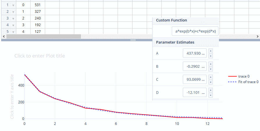
The received signal is well described by the sum of two exponents:
where - reference number.
I selected most of the data (110 sets of values, the train.dat file) for training ( training dataset ) (when loading they are further subjected to randomization - mixing), and a smaller part (40 sets, the test.dat file) for the validation of the neural network ( validation dataset ) - cross-checks in its simplest form (on holdout dataset ).
Neural network structure
The classic direct propagation neural network created will have three layers:
the input layer - from 8 neurons - perceives the points of the voltage curve;
hidden layer - from three neurons;
output layer - from two neurons.
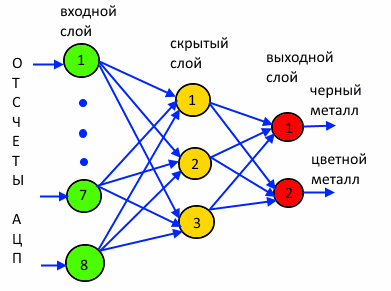
(network "8-3-2")
The Iranians in the above work used two readings (respectively, two input neurons) and three neurons in two hidden layers (the neural network scheme is depicted and described in their article not very clearly).
Neutron state defined as weighted ( - weight) amount input signals (perceived by dendrites) and displacement :
(addition of bias can be represented as an effect of an additional neuron bias)
The state of the neuron is converted to an output signal (at the axon terminals) using the activation function :
The input signals of the neural network arriving at the neurons of the input layer are transmitted to their outputs unchanged, which corresponds to the linear activation function:
For the neurons of the hidden and output layer, a nonlinear activation function, “sigmoid,” is used, or rather its very popular option — the logistic function — with an interval of values (0; 1):
This choice of activation function is great for non-negative ADC counts. But this requires, of course, the normalization of input values - we divide them by 1024, which guarantees a value less than 1.
The Iranians used the hyperbolic tangent as an activation function.
The values of the output neurons of the output layer determine the results of the neural network. The neuron with the maximum output value will indicate the decision (winning class) made by the network: the first class is “ferrous metal”, the second class is “non-ferrous metal”.
The Iranians used three output neurons pointing to iron, copper and lead.
Python - PyTorch , Keras , TensorFlow , CNTK , libraries and frameworks for neural networks are also created for JavaScript - Synaptic , Java - Deeplearning4j , C ++ - CNTK , MATLAB is not far behind.
But for the subsequent “field” use in the metal detector, these frameworks / libraries are of little use, so for a detailed understanding of the process I built my neural network without using additional INS support libraries. Neural network, of course, you can write on BASIC :-). But under the influence of my subjective preferences, I chose Go .
Training and validation of the neural network
When creating a network, weights are initialized with random values in the range (-0.1; 0.1).
I used the stochastic gradient descent ( SGD ) method for network learning.
The neural network performs a single iteration of the learning process, using one of the learning sets provided in sequence. In this case, the forward propagation operation is first performed — the network processes the input set of signals from the training example. Then, based on the obtained solution, the back propagation algorithm is implemented. To update the weights in the learning process, I applied the formula of “vanilla” gradient descent, which uses one hyperparameter - the learning rate coefficient (sometimes denoted by ), i.e. the second popular hyper parameter is not used - factor of the moment ( momentum factor ).
The learning epoch ends after using the entire training data set. After the end of an epoch, the mean square error ( Mean Squared Error ( MSE )) of training is calculated, the neural network is fed a set of values for validation (cross-check on pending data), the mean square of the validation error is determined, the accuracy of predictions ( accuracy ) and the cycle repeats. The cycle stops after reaching the required level of the mean square of the validation error.
After compiling the source code ( nn4md.go file) and launching the executable file, the console displays the learning process — the era number ( Epoch ), the average square of the learning and validation errors ( MSE ), and the prediction accuracy on the data array for validation ( Acc .).
Here is a fragment of such a protocol:
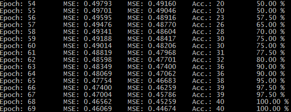
Changing the starting number affects the initial values of the weights of the neural network, which leads to slight differences in the learning process. With a learning rate factor of 0.1, training is completed (when MSE = 0.01 is reached on the test set) in about 300 epochs.
The accuracy of decisions on the data array for validation is 100% (the program gives the number of the winning neuron, starting from 0 - “0” - the first neuron, ferrous metal; “1” - the second neuron, nonferrous metal):
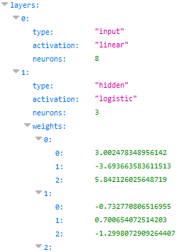
The resulting weights of the neural network after training are saved for later use in a text file nn4md.json in JSON format. By the way, for coding JSON structures on Go it is convenient to use this online tool .
Since the generally accepted and convenient standard for the storage format of neural network settings has not yet been developed (although there is, of course, NNEF - but for such a simple network it is too IMHO ), I used my own format:
Neural Network Testing
And now we are testing a trained neural network on the recognition of new targets ( test dataset ).
Target number 5 (from ferrous metal) :
Curve view:

Value set:
768 224 96 48 14 0 0 0
Target number 6 (from non-ferrous metal) :
Curve view:

Value set:
655 352 254 192 152 124 96 78
Upon completion of training, the program waits for data entry for testing.
Check for target number 5:
Success - “0” - ferrous metal.
And now let's check for target number 6:
Success - “1” - non-ferrous metal.
That turned out to be almost a proof-of-concept .
Data set files, network weights file and source code are available in the repository on GitHub.
One of the most popular options for the design of devices for metal search is a pulse ( pulse induction ( PI )) metal detector — an unpretentious and reliable apparatus (good detection depth, resistance to increased ground mineralization, ability to work in salt water), having various applications from military (traditional users of "impulse") before searching for gold (this hobby is particularly popular in Australia).
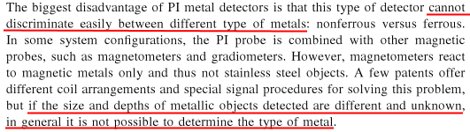
But he also has a significant drawback - great difficulties with discrimination, i.e. determining the type of target, for example, to find out - is it made of ferrous metal or black, or is it possible to distinguish an anti-personnel mine in a plastic case from a handful of metal debris? What is the cause of this problem?
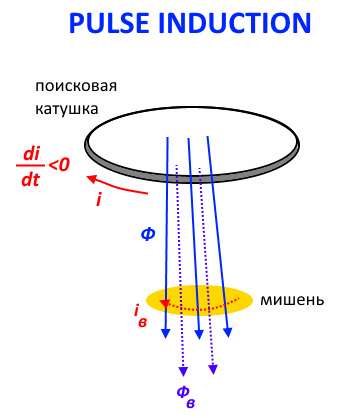
Consider the principle of operation of a pulse metal detector.
The electronic key (usually a MOSFET that can withstand a voltage of several hundred volts — for example, the popular IRF740 is used in this creation by Malaysian engineers, and in this project, based on the programmable analog-digital matrix GreenPAK , the search coil is connected to a power source (battery battery). When a control pulse is applied to the gate of the transistor (usually with a frequency of several tens or hundreds of hertz), the MOSFET opens - the circuit is closed, and a growing (gradually due to the transient process) current flows through the coil. We are waiting for a few tens or hundreds of microseconds of current rise to the desired level and ... breaking the circuit - the control impulse is over. Current through the coil and, accordingly, the magnetic flux the coil decreases sharply (to speed up the process of closing the MOSFET, the control impulse is not supplied directly to the gate, but through a special driver), which, due to the phenomenon of electromagnetic induction, causes the appearance of EMF of self-induction and a sharp increase in voltage on the coil. Then the voltage level on the coil starts to decrease. But if a conducting object (“target”) is located near the coil, then the magnetic flux through the coil decreasing with the current induces eddy currents in this target. These eddy currents create their own magnetic flux. who is trying to maintain the damped magnetic field of the coil. This effect leads to an increase in the voltage decay time at the coil, which is an indicator of the absence or presence of the target (the decision is made either by integrating the signal and estimating the integral value ( a ) or based on the signal values at several points ( b )):
Note : the pulses can be bipolar (for example, the Vallon VMH2 metal detector is a classic device used in demining):
( source )
The average value (constant component) of the magnetic field created by the metal detector is close to zero, which should (as cautiously written in the catalogs, “according to the manufacturer”) prevent undermining when searching for mines reacting to the magnetic field (although, as stated in "Metal detector handbook for humanitarian demining" , with humanitarian demining such an incident is unlikely).
Along with the described variant with one coil, combining the functions of transmitting and receiving, there are pulsed metal detectors with two separate coils. This scheme is applied not only in the field of metal search, but also in flaw detection ( Pulsed Eddy Current (PEC) Testing ) - link 1 , link 2 . In this case, one of the coils ( transmit / drive coil ) serves to excite eddy currents in the target, and the other ( receive / pickup coil ) serves as a magnetic field sensor. This approach makes it possible to analyze the magnetic field not only at the stage of decreasing (after disconnecting the power source from the transmitting coil), but also at the increasing stage (after connecting the power supply to the transmitting coil):
Here is a great description of this technology:
Decay Method for High Purity Metals
Discrimination issue
The problem of recognition of the type of metal arises from the fact that the resulting voltage curve on the coil is influenced by the size and shape of the target, its distance from the coil and electrical (conductivity ) and magnetic (magnetic permeability ) properties of the target material.
Here are a few quotes on this topic:
(source: Ahmet S. Turk, Koksal A. Hocaoglu, Alexey A. Vertiy Subsurface Sensing)
It has been the rule of law that it has been used to detect the metal.( source )
... alter the signal( source )
Many attempts have been made to create pulsed metal detectors capable of distinguishing between iron, silver and copper, but all these attempts have had very limited success. This is due to the physics of the pulse signal.( source )
')
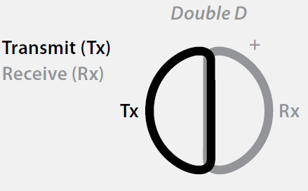
One approach to solving this problem is to use Double-D ( DD ) coils instead of the usual monoloop, for example, in popular Minelab GPX series metal detectors:
( source )
In such a coil, the transmitting ( TX ) and receiving ( RX ) windings are separated:
( source )
In this case, the signal from the target is analyzed not only when decreasing, but also when the current increases in the transmitting coil. But this discrimination is not very reliable:
( source )
But what about the single-loop reel? In many works ( reference 1 reference 2 reference 3 ) it is indicated that the signal in the coil from the target can be represented as a weighted sum of damped exponential signals whose maximum values and time constants are individual and depend on the material, size and shape of the target:
In the work " Discrimination experiments with the US Army's standard metal detector, " it is reported that in experiments conducted by the authors of the article, small objects were well characterized by one exhibitor , and for large objects, two were needed - .
This article indicates that the time constant of the exponential component can be represented as the ratio of equivalent inductance and resistance and gives its expression for a cylinder with a base radius and tall :
This paper presents the expression of the decay time constant of eddy currents for a sphere of radius :
,
Where - the result of solving the equation
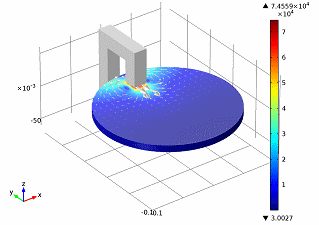
Note : such analytical expressions can be obtained only for simple symmetric bodies. Therefore, to study the eddy currents, you can use software packages for numerical simulation of electromagnetic processes. As an example, the simulation of electromagnetic brakes on eddy currents in the COMSOL Multiphysics package:
( source )
As you can see, the expressions for the time constant together include the magnetic permeability, electrical conductivity and the size of the target. It is not so simple to single out the influence of these factors separately, which is required for discrimination.
In the work already mentioned, it is proposed to use the Bayes classifier to distinguish mines from metal debris (two hypotheses are tested: - garbage, - mine), but this requires additional estimates of the symmetry of the signal, etc. (it is interesting that the composition of the factors used includes the signal energy, estimated as ).
For illustration, I built on the screen of my experimental stand the original design of the voltage graphics on the coil for various targets:
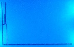
no target:
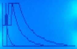
Target number 1 (ferrous metal) at different distances from the coil:
target number 2 (ferrous metal):
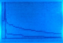
Target number 3 (non-ferrous metal) at different distances from the coil:
Target number 4 (non-ferrous metal):
As can be seen, for ferrous metal targets, due to the greater magnetic permeability, the initial signal level is higher than that for nonferrous metal targets, but the signal decays faster due to lower specific electrical conductivity.
NEUROSET
How, based on these very weak signs, to classify the target, especially when the distance from the target to the metal detector coil is changed? We have a wonderful tool - an artificial neural network. Neural networks play tic-tac-toe , blackjack , poker , predict the weather and quality of wine , calculate the resistance to the movement of agricultural equipment ... So apply the neural network to solve the problem of discrimination!
Proof that this is possible is provided by the article “Improving the performance of PI systems through the use of neural network” by Iranian researchers:
Data for neural network
To fill the data array for learning, validating and testing the neural network, pressing the button on the body of my stand measures 8 points (the number of points chosen empirically) on the voltage curve and outputs ATmega328 ADC samples in symbolic form to the serial port connected to the computer’s USB connector.
In the stand in front of the entrance of the operational amplifier, a diode limiter is turned on, but, as the simulation showed, in the section of interest (with low voltage on the coil), its influence on the voltage value is negligible:
Turning on the logging mode in the terminal program (for example, Tera Term ), we get the “raw” data (for convenience, you can add comments to the Tera Term ). A small utility written on Go converts this data into a format suitable for consumption by the neural network:
i1 i2 ... i8 o1 o2
An example of a string with a set of values:
588 352 312 280 252 240 206 192 0 1
The input data i1 i2 ... i8 are samples of a 10-bit ADC in the range 0 ... 1023.
Output o1 o2 is presented in the form:
“Ferrous metal” ( 1 0), “non-ferrous metal” (0 1 ).
I collected data in the presence of a ferrous metal target near the coil (target No. 1, target No. 2), with a target made from non-ferrous metal (target No. 3, target No. 4), and the targets were located at different distances from the search coil. For further use, data were selected that corresponded to a sufficient signal level — with at least two non-zero values. The data sets corresponding to the overload of the ADC input — containing several maximum possible values (1023) were also discarded:
To illustrate, I performed a regression analysis for one data set:
The received signal is well described by the sum of two exponents:
where - reference number.
I selected most of the data (110 sets of values, the train.dat file) for training ( training dataset ) (when loading they are further subjected to randomization - mixing), and a smaller part (40 sets, the test.dat file) for the validation of the neural network ( validation dataset ) - cross-checks in its simplest form (on holdout dataset ).
Neural network structure
The classic direct propagation neural network created will have three layers:
the input layer - from 8 neurons - perceives the points of the voltage curve;
hidden layer - from three neurons;
output layer - from two neurons.
(network "8-3-2")
The Iranians in the above work used two readings (respectively, two input neurons) and three neurons in two hidden layers (the neural network scheme is depicted and described in their article not very clearly).
Neutron state defined as weighted ( - weight) amount input signals (perceived by dendrites) and displacement :
(addition of bias can be represented as an effect of an additional neuron bias)
The state of the neuron is converted to an output signal (at the axon terminals) using the activation function :
The input signals of the neural network arriving at the neurons of the input layer are transmitted to their outputs unchanged, which corresponds to the linear activation function:
For the neurons of the hidden and output layer, a nonlinear activation function, “sigmoid,” is used, or rather its very popular option — the logistic function — with an interval of values (0; 1):
This choice of activation function is great for non-negative ADC counts. But this requires, of course, the normalization of input values - we divide them by 1024, which guarantees a value less than 1.
The Iranians used the hyperbolic tangent as an activation function.
The values of the output neurons of the output layer determine the results of the neural network. The neuron with the maximum output value will indicate the decision (winning class) made by the network: the first class is “ferrous metal”, the second class is “non-ferrous metal”.
The Iranians used three output neurons pointing to iron, copper and lead.
Python - PyTorch , Keras , TensorFlow , CNTK , libraries and frameworks for neural networks are also created for JavaScript - Synaptic , Java - Deeplearning4j , C ++ - CNTK , MATLAB is not far behind.
But for the subsequent “field” use in the metal detector, these frameworks / libraries are of little use, so for a detailed understanding of the process I built my neural network without using additional INS support libraries. Neural network, of course, you can write on BASIC :-). But under the influence of my subjective preferences, I chose Go .
Training and validation of the neural network
When creating a network, weights are initialized with random values in the range (-0.1; 0.1).
I used the stochastic gradient descent ( SGD ) method for network learning.
The neural network performs a single iteration of the learning process, using one of the learning sets provided in sequence. In this case, the forward propagation operation is first performed — the network processes the input set of signals from the training example. Then, based on the obtained solution, the back propagation algorithm is implemented. To update the weights in the learning process, I applied the formula of “vanilla” gradient descent, which uses one hyperparameter - the learning rate coefficient (sometimes denoted by ), i.e. the second popular hyper parameter is not used - factor of the moment ( momentum factor ).
The learning epoch ends after using the entire training data set. After the end of an epoch, the mean square error ( Mean Squared Error ( MSE )) of training is calculated, the neural network is fed a set of values for validation (cross-check on pending data), the mean square of the validation error is determined, the accuracy of predictions ( accuracy ) and the cycle repeats. The cycle stops after reaching the required level of the mean square of the validation error.
After compiling the source code ( nn4md.go file) and launching the executable file, the console displays the learning process — the era number ( Epoch ), the average square of the learning and validation errors ( MSE ), and the prediction accuracy on the data array for validation ( Acc .).
Here is a fragment of such a protocol:
Changing the starting number affects the initial values of the weights of the neural network, which leads to slight differences in the learning process. With a learning rate factor of 0.1, training is completed (when MSE = 0.01 is reached on the test set) in about 300 epochs.
The accuracy of decisions on the data array for validation is 100% (the program gives the number of the winning neuron, starting from 0 - “0” - the first neuron, ferrous metal; “1” - the second neuron, nonferrous metal):
0 -> 0
0 -> 0
0 -> 0
...
1 -> 1
1 -> 1
1 -> 1
The resulting weights of the neural network after training are saved for later use in a text file nn4md.json in JSON format. By the way, for coding JSON structures on Go it is convenient to use this online tool .
Since the generally accepted and convenient standard for the storage format of neural network settings has not yet been developed (although there is, of course, NNEF - but for such a simple network it is too IMHO ), I used my own format:
Neural Network Testing
And now we are testing a trained neural network on the recognition of new targets ( test dataset ).
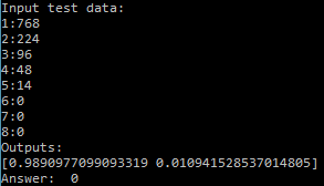
Target number 5 (from ferrous metal) :
Curve view:
Value set:
768 224 96 48 14 0 0 0
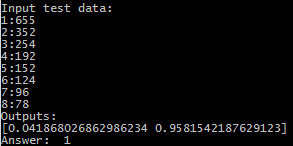
Target number 6 (from non-ferrous metal) :
Curve view:
Value set:
655 352 254 192 152 124 96 78
Upon completion of training, the program waits for data entry for testing.
Check for target number 5:
Success - “0” - ferrous metal.
And now let's check for target number 6:
Success - “1” - non-ferrous metal.
That turned out to be almost a proof-of-concept .
Data set files, network weights file and source code are available in the repository on GitHub.
Source: https://habr.com/ru/post/435884/
All Articles