The theory of happiness. Statistics, as a scientific way to not know anything
I continue to acquaint Habr's readers with chapters from my book “The Theory of Happiness” with the subtitle “Mathematical foundations of the laws of meanness”. This is not a published popular science book, very informally telling how mathematics allows you to look at the world and life of people with a new degree of awareness. It is for those who are interested in science and for those who are interested in life. And since our life is complex and, by and large, unpredictable, the emphasis in the book is mainly on probability theory and mathematical statistics. Here theorems are not proved and the fundamentals of science are not given; this is by no means a textbook, but what is called recreational science. But it is this almost playful approach that allows us to develop intuition, brighten up lectures for students with vivid examples, and, finally, explain to nemathematicians and our children what we found so interesting in our dry science.
This chapter deals with statistics, weather, and even philosophy. Don't be scared, just a little bit. No more than what can be used for tabletalk in a decent society.

')
How often in the summer we plan on our weekends a trip to nature, a walk in the park or a picnic, and then the rain breaks our plans, sharpening us in the house! And it would be okay if this happened once or twice in a season, sometimes it seems that the bad weather is following the weekends, getting on Saturday or Sunday again and again!
A relatively recently published article by Australian researchers: "Weekly cycles of peak temperature and intensity of urban heat islands." She was picked up by the news publications and reprinted the results with the title: “You don’t think! Scientists have found out: the weather is on the weekend, really worse than on weekdays. ” The cited work provides statistics of temperature and precipitation over many years in several cities in Australia, indeed, revealing a decrease in temperature at certain hours of Saturday and Sunday. After that, an explanation is given that relates the local weather to the level of air pollution due to the increasing traffic flow. Shortly before, a similar study was conducted in Germany and led to about the same conclusions.
Agree that a fraction of a degree is a very subtle effect. While complaining about the bad weather on the long-awaited Saturday, we are discussing whether it was a sunny or rainy day, this fact is easier to register, and later to remember, even without possessing accurate instruments. We will conduct our own small research on this topic and get a wonderful result: we can confidently say that we do not know whether day and week are connected in Kamchatka. Research with a negative result usually does not fall on the pages of magazines and news feeds, but it’s important for us to understand on what basis I, in general, can confidently say something about random processes. And in this regard, a negative result becomes no worse than a positive one.
Statistics are accused of the mass of sins: both of lies and possibilities of manipulation and, finally, of incomprehensibility. But I really want to rehabilitate this area of knowledge, to show how difficult the task is for which it is intended and how difficult it is to understand the answer given by statistics.
Probability theory operates with accurate knowledge of random variables in the form of distributions or exhaustive combinatorial calculations. Once again, it is possible to have accurate knowledge of a random variable. But what if this exact knowledge is not available to us, and the only thing we have is observation? The developer of a new drug has some limited number of tests, the creator of the traffic control system has only a series of measurements on a real road, the sociologist has the results of surveys, and he can be sure that answering some questions, the respondents just lied.
It is clear that one observation does not give anything. Two - a little more than nothing, three, four ... one hundred ... how many observations are needed to gain any knowledge of a random quantity, which one could be sure of with mathematical precision? And what kind of knowledge will it be? Most likely, it will be presented in the form of a table or a histogram, making it possible to estimate some parameters of a random variable, they are called statisticians (for example, domain, average or dispersion, asymmetry, etc.). Perhaps, looking at the histogram, one can guess the exact form of the distribution. But attention! - all the results of the observations themselves will be random variables! As long as we do not have accurate knowledge of the distribution, all the results of observations give us only a probabilistic description of a random process! A random description of a random process - still would not get confused here, or even want to confuse intentionally!
What makes mathematical statistics an exact science? Her methods allow us to conclude our ignorance in a well-defined framework and give a computable measure of confidence that within these frameworks our knowledge is consistent with the facts. It is a language in which one can reason about unknown random variables so that the reasoning makes sense. Such an approach is very useful in philosophy, psychology or sociology, where it is very easy to embark on lengthy arguments and discussions without any hope of obtaining positive knowledge and, moreover, on evidence. Literary statistical data processing is devoted to a lot of literature, because it is an absolutely necessary tool for medical professionals, sociologists, economists, physicists, psychologists ... in a word, for all those who scientifically research the so-called “real world”, which differs from the ideal mathematical one only by the degree of our ignorance about it.
Now take another look at the epigraph to this chapter and realize that statistics, which is so scornfully called the third degree of lies, is the only thing that natural sciences have. Is not the main law of the meanness of the universe! All natural laws known to us, from physical to economic, are built on mathematical models and their properties, but they are verified by statistical methods in the course of measurements and observations. In everyday life, our mind makes generalizations and notices patterns, selects and recognizes repetitive images, this is probably the best that the human brain can do. This is exactly what artificial intelligence is taught today. But the mind saves its strength and is inclined to draw conclusions from single observations, without much worrying about the accuracy or validity of these conclusions. On this occasion, there is a remarkable self-consistent statement from Stephen Brasta’s book “Isola”: “Everyone makes general conclusions from one example. At least that's what I do . ” And while we are talking about art, the nature of pets or a discussion of politics, you can not worry about it. However, during the construction of the aircraft, the organization of the airport's dispatch service or the testing of a new drug, it is no longer possible to refer to the fact that “I think so,” “intuition suggests” and “anything can happen in life”. Here you have to limit your mind within the framework of rigorous mathematical methods.
Our book is not a textbook, and we will not study in detail the statistical methods and confine ourselves to only one thing - the technique of testing hypotheses. But I would like to show the course of reasoning and the form of the results characteristic of this area of knowledge. And, perhaps, to some of the readers, the future student, not only it becomes clear why he is tortured by mathematical statistics, all these QQ-diagrams, t-and F-distributions, but another important question comes to mind: how is it possible to know that sure about random occurrence? And what exactly do we find out using statistics?
The main pillars of mathematical statistics are probability theory, the law of large numbers, and the central limit theorem .
The law of large numbers, in a free interpretation, says that a large number of observations of a random variable almost certainly reflects its distribution , so that the observed statistics: mean, variance, and other characteristics tend to exact values corresponding to a random variable. In other words, the histogram of the observed values with an infinite number of data, almost certainly tends to the distribution, which we can consider to be true. It is this law that binds the “domestic” frequency interpretation of probability and the theoretical one, as measures on a probability space.
The central limit theorem, again, in a free interpretation, says that one of the most likely forms of distribution of a random variable is the normal (Gaussian) distribution. The exact formulation sounds different: the average value of a large number of identically distributed real random variables, regardless of their distribution, is described by a normal distribution. This theorem is usually proved by applying the methods of functional analysis, but we will see later that it can be understood and even expanded by introducing the concept of entropy as a measure of the probability of the system state: the normal distribution has the greatest entropy with the least number of restrictions. In this sense, it is optimal when describing an unknown random variable, or a random variable, which is a collection of many other variables, the distribution of which is also unknown.
These two laws form the basis of quantitative assessments of the reliability of our knowledge based on observations. Here we are talking about the statistical confirmation or refutation of the assumption that can be made from some common grounds and a mathematical model. This may seem strange, but in itself, statistics do not produce new knowledge. A set of facts turns into knowledge only after building links between the facts that form a certain structure. It is these structures and relationships that allow making predictions and making general assumptions based on something that goes beyond statistics. Such assumptions are called hypotheses . It's time to recall one of the laws of merphology, Percig's postulate :
The task of mathematical statistics to limit this infinite number, or rather to reduce them to one, and not necessarily true. To move to a more complex (and often more desirable) hypothesis, it is necessary, using observational data, to refute a simpler and more general hypothesis, or to support it and abandon the further development of the theory. The hypothesis often tested in this way is called null , and there is a deep meaning in it.
What can play the role of the null hypothesis? In a certain sense, anything, any statement, but on condition that it can be translated into a measurement language. Most often, the hypothesis is the expected value of a parameter that turns into a random variable during the measurement, or the absence of a relationship (correlation) between two random variables. Sometimes it is assumed the type of distribution, random process, some mathematical model is offered. The classical statement of the question is as follows: do observations allow one to reject the null hypothesis or not? More precisely, with what degree of confidence can we say that observations cannot be obtained on the basis of the null hypothesis? In this case, if we could not rely on statistical data to prove that the null hypothesis is false, then it is assumed to be true.
And here you might think that researchers are forced to make one of the classic logical errors, which bears the resounding Latin name ad ignorantiam. This is the argument of the truth of some statement, based on the absence of evidence of its falsity. A classic example is the words spoken by Senator Joseph McCarthy when he was asked to present facts to support the accusation that a certain person is a communist: “I have some information on this issue, except for the general statement of the competent authorities that there is nothing in his file , to exclude his connection with the Communists . " Or even brighter: "The snowman exists, because no one has proven otherwise . " Identifying the difference between a scientific hypothesis and similar tricks is the subject of a whole field of philosophy: the methodology of scientific knowledge . One of its striking results is the criterion of falsifiability , put forward by the remarkable philosopher Karl Popper in the first half of the 20th century. This criterion is designed to separate scientific knowledge from unscientific, and, at first glance, it seems paradoxical:
What is not the law of meanness! It turns out that any scientific theory is automatically potentially incorrect, and a theory that is true “by definition” cannot be considered scientific. Moreover, such criteria as mathematics and logic do not satisfy this criterion. However, they are referred not to the natural sciences, but to the formal ones , which do not require checking for falsifiability. And if we add another result of the same time to this: Gödel’s principle of incompleteness , which asserts that within any formal system one can formulate an assertion that can neither be proved nor disproved, then it may become unclear why, in general, to be engaged in the whole science. However, it is important to understand that Popper’s falsifiability principle says nothing about the truth of a theory, but only whether it is scientific or not. It can help determine whether a certain theory gives a language in which it makes sense to talk about the world or not.
But still, why, if we cannot reject the hypothesis on the basis of statistical data, are we entitled to accept it as true? The fact is that the statistical hypothesis is not taken from the desire of the researcher or his preferences; it must flow from any general formal laws. For example, from the Central Limit Theorem, or from the principle of maximum entropy. These laws correctly reflect the degree of our ignorance , without unnecessarily adding unnecessary assumptions or hypotheses. In a sense, this is a direct use of the famous philosophical principle known as Occam's razor :
Thus, when we accept the null hypothesis, based on the absence of its refutation, we formally and honestly show that as a result of the experiment, the degree of our ignorance remained at the same level . In the example with the snowman, explicitly or implicitly, but the opposite is assumed: the lack of evidence that this mysterious creature does not exist seems to be something that can increase the degree of our knowledge about it.
In general, from the point of view of the principle of falsifiability, any statement about the existence of something is unscientific, because the absence of evidence does not prove anything. At the same time, the statement about the absence of something can be easily refuted by providing a copy, indirect evidence, or by proving the existence by construction. And in this sense, a statistical hypothesis test analyzes the statements about the absence of the desired effect and can provide, in a certain sense, an exact refutation of this statement. This is precisely what fully justifies the term “null hypothesis”: it contains the necessary minimum knowledge of the system.
It is very important to emphasize that if the statistics suggest that the null hypothesis can be rejected, this does not mean that we thereby proved the truth of any alternative hypothesis. Statistics should not be confused with logic, therein lies a lot of subtle errors, especially when conditional probabilities for dependent events come into play. For example: it is very unlikely that a person can be Pope ( s i m 1 / 7 bn) follow from this that Pope John Paul II was not a man? The statement seems absurd, but, unfortunately, such an "obvious" conclusion is just as wrong: the test showed that the mobile test for alcohol content in the blood gives no more1 % of both false positive and false negative results, therefore, in98 % of cases, he correctly identify a drunk driver. Let's test1000 drivers and let100 of them will be really drunk. As a result, we get900 × 1 % = 9 false positives and100 × 1 % = 1 false negative result: that is, for one drunkard who missed, there would be nine innocently accused random drivers. What is not the law of meanness! Parity will only be observed if the proportion of drunk drivers equals1 / 2 , or if the ratio of the fraction of false positive and false negative results will be close to the actual relative to sober drunk drivers. Moreover, the more sober the nation being surveyed, the more unfair the application of the device described by us!Here we are faced withdependent events. Remember, in the Kolmogorov definition of probability, we talked about the method of adding the probability of combining events: the probability of combining two events is equal to the sum of their probabilities minus the probability of their intersection. However, how the probability of the intersection of events is calculated, these definitions do not speak. To do this, a new concept is introduced: theconditional probabilityand the dependence of events on each other come to the fore.
The probability of intersection of events A and B is defined as the product of the probability of the event B and the probability of the event A , if you know what happened eventB :
Thus, we complete the formal definition of probability, begun in the first chapter.
The intersection is a commutative operation, i.e.P ( A ∩ B ) = P ( B ∩ A ) . This immediately follows the Bayes theorem:
In our example with drivers and an alcohol test, we have events:A - the driver is drunk,B - the test gave a positive result. Probabilities:P ( A ) = 0.1 - the probability that the driver is stopped is drunk;P ( B | A ) = 99 % - the probability that the test will give a positive result, if it is known that the driver is drunk (excluded1 % false negative),P ( A | B ) = 99 % - the probability that the test is drunk, if the test gave a positive result (excluded1 false positive results). CalculateP ( B ) - probability to get a positive test result on the road:
These examples are thoroughly analyzed by medical test students or legal practitioners. But, I am afraid that journalists or politicians are not taught either mathematical statistics or probability theory, but they willingly appeal to statistical data, freely interpret them and carry the resulting "knowledge" to the masses. Therefore, I urge my reader: I figured out the math myself, help me figure out another! I see no other antidote to ignorance.
We will consider and put into practice only one of the many statistical methods: the testing of statistical hypotheses. For those who have already connected their lives with the natural or social sciences in these examples there will not be something shockingly new.
Suppose we repeatedly measure a random variable with an average value m u and standard deviation s i g m a .According to the Central Limit Theorem, the observed average value will be distributed normally. It follows from the law of large numbers that its average will tend to m u , and from the properties of the normal distribution it follows that aftern measurements, the observed variance of the mean will decrease asσ / √n . The standard deviation can be considered as an absolute error of measurement of the mean, the relative error will be equal to δ = σ / ( √n μ) . These are very general conclusions that do not depend on sufficiently large n from the specific form of the distribution of the random variable under study. They follow two useful rules (not laws):1. Minimum number of tests
n should be dictated by the desired relative errorδ . However, if
m u . Then, if the observed average does not exceed the limits μ ± 2 σ / √n , then the probability that the null hypothesis is true will be at least95 % .
If replaced in these rules 2 σ on 3 σ , then the degree of confidence will increase to99.7 % , this is a very strong rule3 σ , which in physical sciences separates the assumptions from the experimentally established fact. It will be useful for us to consider the application of these rules to the Bernoulli distribution, which describes a random variable that takes exactly two values, conventionally called “success” and “failure”, with a given probability of success.
p . In this case μ = p and σ = √p ( 1 - p ) , so that for the required number of experiments and the confidence interval we get
Rule 2 σfor the Bernoulli distribution can be used to determine the confidence interval when constructing histograms. In essence, each histogram bar represents a random variable with two values: “hit” - “missed”, where the probability of hitting corresponds to the simulated probability function. As a demonstration, we will generate a set of samples for three distributions: uniform, geometric, and normal, after which we compare the estimates of the spread of the observed data with the observed spread. And here we again see echoes of the central limit theorem, manifested in the fact that the distribution of data around the average values in histograms is close to normal. However, near zero, the scatter becomes asymmetric and approaches another very likely distribution, the exponential. This example shows well what I meantsaying that in statistics we are dealing with random values of parameters of a random variable.
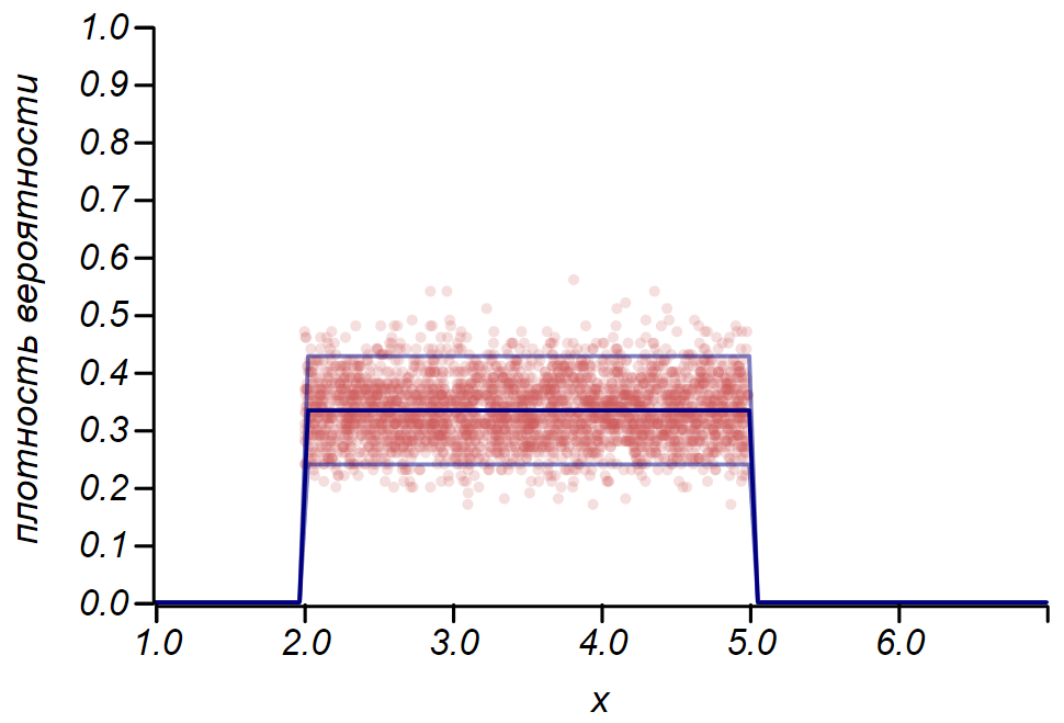
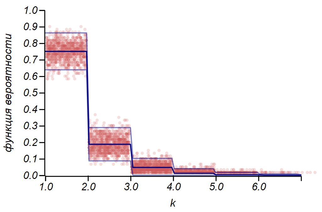
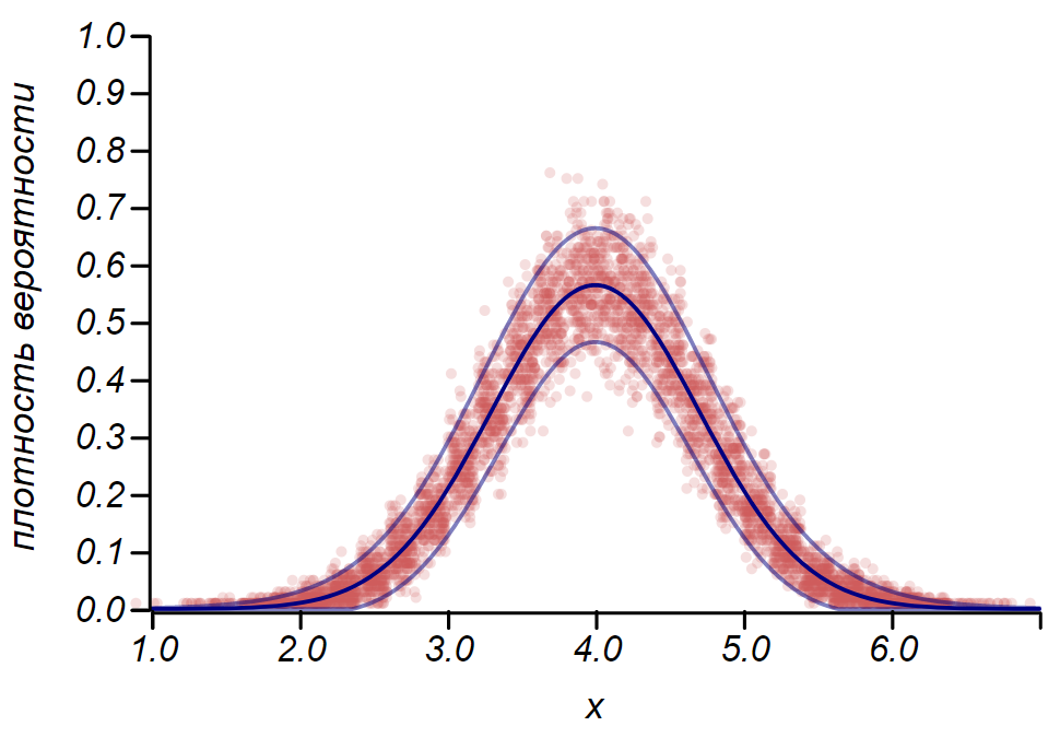 Example showing the ratio of the scatter estimate made according to the rule 2 σ and the observed scatter for three random variables.
It is important to understand that the rules2 σ and even3 σ does not save us from mistakes. They do not guarantee the truth of any statement, they are not evidence. Statistics limit the degree of distrust of the hypothesis, and nothing more. The mathematician and author of the excellent course of probability theory Gian-Carlo Roth, at his lectures at MIT, gave this example. Imagine a scientific journal, the editorial staff of which made a volitional decision: to accept for publication only articles with positive results that satisfy the rule.
2 σ or stricter. At the same time, the editorial column states that readers can be confident that with probability95 % of the reader will not find the wrong result on the pages of this magazine! Alas, this statement is easily refuted by the same reasoning that led us to a gross injustice when testing drivers for alcohol. Let be1000 researchers subjected to experience1000 hypotheses, of which only some part is true, say,10 % . Based on the meaning of hypothesis testing, one can expect that 900 × 0.05 = 45 of the incorrect hypotheses will not be mistakenly rejected, and will be included in the journal along with100 × 0.95 = 95 correct results. Total of130 results, a good third would be wrong! This example perfectly demonstrates our domestic law of meanness, which has not yet entered into the anthology of merphology,Chernomyrdin's law:
It is easy to get a general estimate of the proportion of incorrect results that will be included in the journal issues, assuming that the proportion of correct hypotheses is equal 0 < α < 1 and the probability of making an erroneous hypothesis isp :
 Estimation of the share of publications containing deliberately incorrect results when adopting various criteria for testing hypotheses. It can be seen that to accept hypotheses by the rule 2 σ may be risky, while the criterion 4 σ can already be considered very strong.
Of course, we don't know that. a l p h a , and we will never know, but it is obviously less than one, which means, in any case, the statement from the editorial column cannot be taken seriously. You can limit yourself to a rigid framework of the criterion. 4 s i g m a , but it requires a very large number of tests. This means that it is necessary to increase the proportion of correct hypotheses in the set of possible assumptions. This is what the standard approaches of the scientific method of knowledge are aimed at - the logical consistency of hypotheses, their consistency with facts and theories that have proved their applicability, reliance on mathematical models and critical thinking.
At the beginning of the chapter we talked about the fact that weekends and bad weather coincide more often than we would like. Let's try to complete this study. Every rainy day can be viewed as the observation of a random variable — a day of the week that obeys the Bernoulli distribution with probability 1 / 7 . We take as the null hypothesis the assumption that all days of the week are the same in terms of weather and it can rain in any of them equally likely. We have two weekends, in total, we get the expected probability of coincidence of a bad weather day and a holiday equal to 2 / $ , this value will be a parameter of the Bernoulli distribution. How often does it rain? At different times of the year, of course, in different ways, but in Petropavlovsk-Kamchatsky, on average, there are ninety rainy or snowy days per year. So the flow of precipitation days has an intensity of about 90/365 approx1/4 . Let's calculate how many rainy weekends we have to register in order to be sure that there is some pattern. The results are shown in the table.
What do these numbers say? If it seems to you that that year in a row there was no “summer”, that the evil fate is haunting your weekend, sending rain on them, you can check and confirm it. However, during the summer, evil rock can only be caught if more than two-fifths of the weekend turns out to be rainy. The null hypothesis suggests that only a quarter of the weekend should coincide with inclement weather. For five years of observations, it is already possible to hope to notice subtle deviations beyond the limits of 5% and, if necessary, proceed to their explanation.
I used the school weather diary, which was conducted from 2014 to 2018, and found out what happened during these five years. 459 rainy days of them 141 come on the weekend. This is indeed more than the expected number on 11 days, but significant deviations begin with 19 days, so this, as we said in childhood: "does not count." This is how the data series and the histogram look, showing the distribution of the weather by days of the week. Horizontal lines on the histogram indicate the interval in which a random deviation from a uniform distribution can be observed with the same amount of data.
The initial data series and the distribution of bad days by days of the week, obtained from five years of observations.
It can be seen that since Friday, there is indeed an increase in the number of days with bad weather. But to find the reason for this growth, the prerequisites are not enough: the same result can be obtained simply by going through random numbers. Conclusion: for five years of weather observation, I have accumulated almost two thousand records, but I did not learn anything new about the distribution of weather by days of the week.
When looking at the diary entries, it is clearly striking that bad weather does not come one by one, but two or three-day periods, or even weekly cyclones. Does it somehow affect the result? You can try to take this observation into account, and assume that it rains an average of two days (in fact, 1.7 days), then the probability to cut off the weekend increases to 3/7 . With such a probability, the expected number of matches for five years should be 195 pm21 that is from 174 before 216 time. Observed value 141 does not fall within this range, which means that the hypothesis of the effect of double weather days can be safely rejected. Did we learn something new? Yes, we learned: it would seem that the obvious feature of the process does not entail any effect. This is worth considering, and we will do it a little later. But the main conclusion: there are no reasons to consider any more subtle effects, since observations and, most importantly, their number, consistently speak in favor of the simplest explanation.
But our discontent is caused not by five-year or even annual statistics, human memory is not so long. It's a shame when it rains over the weekend three or four times in a row! How often can this be observed? Especially if you remember that the nasty weather does not come alone. The task can be formulated as: "What is the probability that n Weekend in a row will be rainy? ”It is reasonable to assume that bad days form a Poisson stream with intensity 1/4 . This means that, on average, a quarter of the days of any period will be bad weather. Observing only the weekends, we should not change the intensity of the flow and from all the weekends the bad weather should make up, on average, also a quarter. So, we put forward the null hypothesis: the Poisson flow of bad weather, with a known parameter, and therefore, the intervals between Poisson events are described by an exponential distribution. We are interested in discrete intervals: 0, 1, 2, 3 of the day, etc., so we can use the discrete analogue of the exponential distribution — the geometric distribution with the parameter 1/4 . The figure shows that we have succeeded and it is clear that the assumption that we are observing the Poisson process has no reason to reject.
The observed distribution of the lengths of the failed output chains is theoretical. The thin line shows the tolerances for the number of observations that we have.
One may ask, such a question: how many years it is necessary to conduct observations, in order that we notice the difference in 11 days could you confidently confirm or reject as random rejection? It is easy to calculate: the observed probability 141/459=$0.30 different from expected 2/7=0.286 on 0.02 . To fix the difference in hundredths, an absolute error is required, not exceeding 0.005 , what is 1.75% from the measured value. From here we obtain the required sample size. n geq(4 cdot5/7)/(0.01752 cdot2/7) approx$3200 rainy days. It will take about 4 cdot32000/365 approx360 years of continuous meteorological observations, because only every fourth day it rains or snows. Alas, this is more than the time that Kamchatka is in Russia, so I have no chance to find out how things are “in fact”. Especially if we take into account that during this time the climate has changed dramatically - from the Little Ice Age, nature emerged at the next optimum.
So how did Australian researchers manage to fix the deviation of temperature in a fraction of a degree, and why does it make sense to consider this study? The fact is that they used hourly temperature data that was not “thinned out” by any random process. So for 30 years of meteorological observations, it was possible to accumulate more than a quarter of a million counts, which makes it possible to reduce the standard deviation of the average 500 times relative to standard daily temperature deviation. This is quite enough to talk about accuracy in tenths of a degree. In addition, the authors used another beautiful method confirming the existence of a time cycle: random mixing of the time series. Such mixing preserves statistical properties, such as flow intensity, but “erases” temporal patterns, making the process truly Poisson. Comparison of the set of synthetic series and the experimental one makes sure that the observed deviations from the Poisson process are significant. In the same way, the seismologist A. A. Gusev showed that earthquakes in an area form a kind of self-similar flow with clustering properties. This means that earthquakes tend to cluster in time, forming a very unpleasant stream seals. Later it turned out that the sequence of large volcanic eruptions has the same property.
Of course, the weather, like earthquakes, cannot be described by the Poisson process - these are dynamic processes in which the current state is a function of the previous ones. Why do our weekend weather observations speak in favor of a simple stochastic model? The fact is that we map the regular process of precipitation formation to a set of seven days, or, speaking in the language of mathematics, to a system of residues modulo seven . This projection process is capable of generating chaos from well-ordered data series. Hence, for example, there is a visible randomness in the sequence of digits of the decimal notation of the majority of real numbers.
We have already spoken about rational numbers, those that are expressed as integer fractions. They have an internal structure, which is determined by two numbers: the numerator and the denominator. But when writing in decimal form, one can observe jumps from regularity in the representation of such numbers as 1/2=0.5 overline0 , or 1/3=0. Overline3 until periodic repetition, already completely disordered sequences in such numbers as 1/17=0. Overline0588235294117647 . Irrational numbers do not have a finite or periodic record in decimal form, and in this case chaos reigns in the sequence of numbers. But this does not mean that there is no order in these numbers! For example, the first irrational number met by mathematicians sqrt2 in decimal notation generates a chaotic set of numbers. However, on the other hand, this number can be represented as an infinite continued fraction:
Continued fractions with repeating coefficients are written briefly, like periodic decimal fractions, for example: sqrt2=[1, bar2] , sqrt3=[1, overline1,2] . The famous golden section in this sense is the simplest arranged irrational number: varphi=[1, bar1] . All rational numbers are represented as finite continued fractions, some irrational - as infinite, but periodic, they are called algebraic , the same that do not have a finite notation even in this form - transcendental . The most famous of the transcendental is the number pi it creates chaos both in decimal notation and in the form of a continued fraction: pi approx[3,7,15,1,292,1,1,1,1,1,1,3,1,14,2,1,...] . But the Euler number e while remaining transcendental, in the form of a continued fraction, it exhibits an internal structure hidden in the decimal notation: e approx[2,1,2,1,1,4,1,1,6,1,1,8,1,1,10,...] .
Probably not one mathematician, starting with Pythagoras, suspected the world of cunning, discovering what is necessary, such a fundamental number pi has such an elusively complex chaotic structure. Of course, it can be presented in the form of sums of quite elegant numerical series, but these series do not directly speak about the nature of this number and they are not universal. I believe that the mathematicians of the future will open up some new representation of numbers, as universal as continued fractions, which will reveal the strict order hidden by nature in the number.
The results of this chapter are, for the most part, negative. And as an author who wants to surprise the reader with hidden patterns and unexpected discoveries, I wondered whether to include it in a book. But our conversation about the weather went into a very important topic - about the value and meaningfulness of the natural science approach.
One wise girl, Sonya Shatalova, looking at the world through the prism of autism, at the age of ten gave a very concise and precise definition: “Science is a system of knowledge based on doubt . ” The real world is unsteady and strives to hide behind the complexity, apparent randomness and unreliability of measurements. Doubt in the natural sciences is inevitable. Mathematics seems to be the realm of certainty, in which, it seems, you can forget about doubt. And it is very tempting to hide behind the walls of this kingdom; consider instead of the difficult to recognize world models that can be thoroughly investigated; read and calculate, the benefit of the formula ready to digest anything. But nevertheless, mathematics is a science and doubt in it is a deep inner honesty, which does not give rest until the mathematical construction is cleared of additional assumptions and unnecessary hypotheses. In the realm of mathematics, they speak a complex but well-proportioned language suitable for reasoning about the real world. It is very important to get acquainted with this language a little, in order not to let the numbers impersonate statistics, not to let the facts pretend to be knowledge, but to oppose real science to ignorance and manipulation.
Published chapters:
• Introduction to Merphology
• Accidents are random?
• dizzying flight of butter sandwich
• Statistics, as a scientific way to not know anything
• The law of watermelon peel and the normality of abnormality
• The law of the zebra and the queue
• The curse of the director and damn printers
• Thermodynamics of class inequality
• Accidents are random?
• dizzying flight of butter sandwich
• Statistics, as a scientific way to not know anything
• The law of watermelon peel and the normality of abnormality
• The law of the zebra and the queue
• The curse of the director and damn printers
• Thermodynamics of class inequality
This chapter deals with statistics, weather, and even philosophy. Don't be scared, just a little bit. No more than what can be used for tabletalk in a decent society.
')
Figures are deceptive, especially when I do them myself; on this occasion, the statement attributed to Disraeli is true: "There are three types of lies: lies, impudent lies and statistics."
Mark Twain
How often in the summer we plan on our weekends a trip to nature, a walk in the park or a picnic, and then the rain breaks our plans, sharpening us in the house! And it would be okay if this happened once or twice in a season, sometimes it seems that the bad weather is following the weekends, getting on Saturday or Sunday again and again!
A relatively recently published article by Australian researchers: "Weekly cycles of peak temperature and intensity of urban heat islands." She was picked up by the news publications and reprinted the results with the title: “You don’t think! Scientists have found out: the weather is on the weekend, really worse than on weekdays. ” The cited work provides statistics of temperature and precipitation over many years in several cities in Australia, indeed, revealing a decrease in temperature at certain hours of Saturday and Sunday. After that, an explanation is given that relates the local weather to the level of air pollution due to the increasing traffic flow. Shortly before, a similar study was conducted in Germany and led to about the same conclusions.
Agree that a fraction of a degree is a very subtle effect. While complaining about the bad weather on the long-awaited Saturday, we are discussing whether it was a sunny or rainy day, this fact is easier to register, and later to remember, even without possessing accurate instruments. We will conduct our own small research on this topic and get a wonderful result: we can confidently say that we do not know whether day and week are connected in Kamchatka. Research with a negative result usually does not fall on the pages of magazines and news feeds, but it’s important for us to understand on what basis I, in general, can confidently say something about random processes. And in this regard, a negative result becomes no worse than a positive one.
Word in defense of statistics
Statistics are accused of the mass of sins: both of lies and possibilities of manipulation and, finally, of incomprehensibility. But I really want to rehabilitate this area of knowledge, to show how difficult the task is for which it is intended and how difficult it is to understand the answer given by statistics.
Probability theory operates with accurate knowledge of random variables in the form of distributions or exhaustive combinatorial calculations. Once again, it is possible to have accurate knowledge of a random variable. But what if this exact knowledge is not available to us, and the only thing we have is observation? The developer of a new drug has some limited number of tests, the creator of the traffic control system has only a series of measurements on a real road, the sociologist has the results of surveys, and he can be sure that answering some questions, the respondents just lied.
It is clear that one observation does not give anything. Two - a little more than nothing, three, four ... one hundred ... how many observations are needed to gain any knowledge of a random quantity, which one could be sure of with mathematical precision? And what kind of knowledge will it be? Most likely, it will be presented in the form of a table or a histogram, making it possible to estimate some parameters of a random variable, they are called statisticians (for example, domain, average or dispersion, asymmetry, etc.). Perhaps, looking at the histogram, one can guess the exact form of the distribution. But attention! - all the results of the observations themselves will be random variables! As long as we do not have accurate knowledge of the distribution, all the results of observations give us only a probabilistic description of a random process! A random description of a random process - still would not get confused here, or even want to confuse intentionally!
What makes mathematical statistics an exact science? Her methods allow us to conclude our ignorance in a well-defined framework and give a computable measure of confidence that within these frameworks our knowledge is consistent with the facts. It is a language in which one can reason about unknown random variables so that the reasoning makes sense. Such an approach is very useful in philosophy, psychology or sociology, where it is very easy to embark on lengthy arguments and discussions without any hope of obtaining positive knowledge and, moreover, on evidence. Literary statistical data processing is devoted to a lot of literature, because it is an absolutely necessary tool for medical professionals, sociologists, economists, physicists, psychologists ... in a word, for all those who scientifically research the so-called “real world”, which differs from the ideal mathematical one only by the degree of our ignorance about it.
Now take another look at the epigraph to this chapter and realize that statistics, which is so scornfully called the third degree of lies, is the only thing that natural sciences have. Is not the main law of the meanness of the universe! All natural laws known to us, from physical to economic, are built on mathematical models and their properties, but they are verified by statistical methods in the course of measurements and observations. In everyday life, our mind makes generalizations and notices patterns, selects and recognizes repetitive images, this is probably the best that the human brain can do. This is exactly what artificial intelligence is taught today. But the mind saves its strength and is inclined to draw conclusions from single observations, without much worrying about the accuracy or validity of these conclusions. On this occasion, there is a remarkable self-consistent statement from Stephen Brasta’s book “Isola”: “Everyone makes general conclusions from one example. At least that's what I do . ” And while we are talking about art, the nature of pets or a discussion of politics, you can not worry about it. However, during the construction of the aircraft, the organization of the airport's dispatch service or the testing of a new drug, it is no longer possible to refer to the fact that “I think so,” “intuition suggests” and “anything can happen in life”. Here you have to limit your mind within the framework of rigorous mathematical methods.
Our book is not a textbook, and we will not study in detail the statistical methods and confine ourselves to only one thing - the technique of testing hypotheses. But I would like to show the course of reasoning and the form of the results characteristic of this area of knowledge. And, perhaps, to some of the readers, the future student, not only it becomes clear why he is tortured by mathematical statistics, all these QQ-diagrams, t-and F-distributions, but another important question comes to mind: how is it possible to know that sure about random occurrence? And what exactly do we find out using statistics?
Three pillars of statistics
The main pillars of mathematical statistics are probability theory, the law of large numbers, and the central limit theorem .
The law of large numbers, in a free interpretation, says that a large number of observations of a random variable almost certainly reflects its distribution , so that the observed statistics: mean, variance, and other characteristics tend to exact values corresponding to a random variable. In other words, the histogram of the observed values with an infinite number of data, almost certainly tends to the distribution, which we can consider to be true. It is this law that binds the “domestic” frequency interpretation of probability and the theoretical one, as measures on a probability space.
The central limit theorem, again, in a free interpretation, says that one of the most likely forms of distribution of a random variable is the normal (Gaussian) distribution. The exact formulation sounds different: the average value of a large number of identically distributed real random variables, regardless of their distribution, is described by a normal distribution. This theorem is usually proved by applying the methods of functional analysis, but we will see later that it can be understood and even expanded by introducing the concept of entropy as a measure of the probability of the system state: the normal distribution has the greatest entropy with the least number of restrictions. In this sense, it is optimal when describing an unknown random variable, or a random variable, which is a collection of many other variables, the distribution of which is also unknown.
These two laws form the basis of quantitative assessments of the reliability of our knowledge based on observations. Here we are talking about the statistical confirmation or refutation of the assumption that can be made from some common grounds and a mathematical model. This may seem strange, but in itself, statistics do not produce new knowledge. A set of facts turns into knowledge only after building links between the facts that form a certain structure. It is these structures and relationships that allow making predictions and making general assumptions based on something that goes beyond statistics. Such assumptions are called hypotheses . It's time to recall one of the laws of merphology, Percig's postulate :
The number of reasonable hypotheses explaining any given phenomenon is infinite.
The task of mathematical statistics to limit this infinite number, or rather to reduce them to one, and not necessarily true. To move to a more complex (and often more desirable) hypothesis, it is necessary, using observational data, to refute a simpler and more general hypothesis, or to support it and abandon the further development of the theory. The hypothesis often tested in this way is called null , and there is a deep meaning in it.
What can play the role of the null hypothesis? In a certain sense, anything, any statement, but on condition that it can be translated into a measurement language. Most often, the hypothesis is the expected value of a parameter that turns into a random variable during the measurement, or the absence of a relationship (correlation) between two random variables. Sometimes it is assumed the type of distribution, random process, some mathematical model is offered. The classical statement of the question is as follows: do observations allow one to reject the null hypothesis or not? More precisely, with what degree of confidence can we say that observations cannot be obtained on the basis of the null hypothesis? In this case, if we could not rely on statistical data to prove that the null hypothesis is false, then it is assumed to be true.
And here you might think that researchers are forced to make one of the classic logical errors, which bears the resounding Latin name ad ignorantiam. This is the argument of the truth of some statement, based on the absence of evidence of its falsity. A classic example is the words spoken by Senator Joseph McCarthy when he was asked to present facts to support the accusation that a certain person is a communist: “I have some information on this issue, except for the general statement of the competent authorities that there is nothing in his file , to exclude his connection with the Communists . " Or even brighter: "The snowman exists, because no one has proven otherwise . " Identifying the difference between a scientific hypothesis and similar tricks is the subject of a whole field of philosophy: the methodology of scientific knowledge . One of its striking results is the criterion of falsifiability , put forward by the remarkable philosopher Karl Popper in the first half of the 20th century. This criterion is designed to separate scientific knowledge from unscientific, and, at first glance, it seems paradoxical:
A theory or hypothesis can be considered scientific only if there is, even if hypothetically, a way to refute it.
What is not the law of meanness! It turns out that any scientific theory is automatically potentially incorrect, and a theory that is true “by definition” cannot be considered scientific. Moreover, such criteria as mathematics and logic do not satisfy this criterion. However, they are referred not to the natural sciences, but to the formal ones , which do not require checking for falsifiability. And if we add another result of the same time to this: Gödel’s principle of incompleteness , which asserts that within any formal system one can formulate an assertion that can neither be proved nor disproved, then it may become unclear why, in general, to be engaged in the whole science. However, it is important to understand that Popper’s falsifiability principle says nothing about the truth of a theory, but only whether it is scientific or not. It can help determine whether a certain theory gives a language in which it makes sense to talk about the world or not.
But still, why, if we cannot reject the hypothesis on the basis of statistical data, are we entitled to accept it as true? The fact is that the statistical hypothesis is not taken from the desire of the researcher or his preferences; it must flow from any general formal laws. For example, from the Central Limit Theorem, or from the principle of maximum entropy. These laws correctly reflect the degree of our ignorance , without unnecessarily adding unnecessary assumptions or hypotheses. In a sense, this is a direct use of the famous philosophical principle known as Occam's razor :
What can be done on the basis of a smaller number of assumptions should not be done on the basis of a larger one.
Thus, when we accept the null hypothesis, based on the absence of its refutation, we formally and honestly show that as a result of the experiment, the degree of our ignorance remained at the same level . In the example with the snowman, explicitly or implicitly, but the opposite is assumed: the lack of evidence that this mysterious creature does not exist seems to be something that can increase the degree of our knowledge about it.
In general, from the point of view of the principle of falsifiability, any statement about the existence of something is unscientific, because the absence of evidence does not prove anything. At the same time, the statement about the absence of something can be easily refuted by providing a copy, indirect evidence, or by proving the existence by construction. And in this sense, a statistical hypothesis test analyzes the statements about the absence of the desired effect and can provide, in a certain sense, an exact refutation of this statement. This is precisely what fully justifies the term “null hypothesis”: it contains the necessary minimum knowledge of the system.
How to confuse statistics and how to unravel
It is very important to emphasize that if the statistics suggest that the null hypothesis can be rejected, this does not mean that we thereby proved the truth of any alternative hypothesis. Statistics should not be confused with logic, therein lies a lot of subtle errors, especially when conditional probabilities for dependent events come into play. For example: it is very unlikely that a person can be Pope ( s i m 1 / 7 bn) follow from this that Pope John Paul II was not a man? The statement seems absurd, but, unfortunately, such an "obvious" conclusion is just as wrong: the test showed that the mobile test for alcohol content in the blood gives no more1 % of both false positive and false negative results, therefore, in98 % of cases, he correctly identify a drunk driver. Let's test1000 drivers and let100 of them will be really drunk. As a result, we get900 × 1 % = 9 false positives and100 × 1 % = 1 false negative result: that is, for one drunkard who missed, there would be nine innocently accused random drivers. What is not the law of meanness! Parity will only be observed if the proportion of drunk drivers equals1 / 2 , or if the ratio of the fraction of false positive and false negative results will be close to the actual relative to sober drunk drivers. Moreover, the more sober the nation being surveyed, the more unfair the application of the device described by us!Here we are faced withdependent events. Remember, in the Kolmogorov definition of probability, we talked about the method of adding the probability of combining events: the probability of combining two events is equal to the sum of their probabilities minus the probability of their intersection. However, how the probability of the intersection of events is calculated, these definitions do not speak. To do this, a new concept is introduced: theconditional probabilityand the dependence of events on each other come to the fore.
The probability of intersection of events A and B is defined as the product of the probability of the event B and the probability of the event A , if you know what happened eventB :
P ( A ∩ B ) = P ( B ) P ( A | B ) .
You can now determine the independence of events in three equivalent ways: Events A and B are independent ifP ( A | B ) = P ( A ) , orP ( B | A ) = P ( B ) , orP ( A ∩ B ) = P ( A ) P ( B ) .
Thus, we complete the formal definition of probability, begun in the first chapter.
The intersection is a commutative operation, i.e.P ( A ∩ B ) = P ( B ∩ A ) . This immediately follows the Bayes theorem:
P ( A | B ) P ( B ) = P ( B | A ) P ( A ) ,
which can be used to calculate conditional probabilities.
In our example with drivers and an alcohol test, we have events:A - the driver is drunk,B - the test gave a positive result. Probabilities:P ( A ) = 0.1 - the probability that the driver is stopped is drunk;P ( B | A ) = 99 % - the probability that the test will give a positive result, if it is known that the driver is drunk (excluded1 % false negative),P ( A | B ) = 99 % - the probability that the test is drunk, if the test gave a positive result (excluded1 false positive results). CalculateP ( B ) - probability to get a positive test result on the road:
P ( B ) = P ( A ) P ( A | B )P ( B | A ) =P(A)=0.1
Now our reasoning has become formalized and, who knows, perhaps, for someone more understandable. The concept of conditional probability allows logical reasoning in the language of probability theory. Not surprisingly, the Bayes theorem has found wide application in decision theory, in pattern recognition systems, in spam filters, programs that test plagiarism tests, and in many other information technologies.
These examples are thoroughly analyzed by medical test students or legal practitioners. But, I am afraid that journalists or politicians are not taught either mathematical statistics or probability theory, but they willingly appeal to statistical data, freely interpret them and carry the resulting "knowledge" to the masses. Therefore, I urge my reader: I figured out the math myself, help me figure out another! I see no other antidote to ignorance.
We measure our gullibility
We will consider and put into practice only one of the many statistical methods: the testing of statistical hypotheses. For those who have already connected their lives with the natural or social sciences in these examples there will not be something shockingly new.
Suppose we repeatedly measure a random variable with an average value m u and standard deviation s i g m a .According to the Central Limit Theorem, the observed average value will be distributed normally. It follows from the law of large numbers that its average will tend to m u , and from the properties of the normal distribution it follows that aftern measurements, the observed variance of the mean will decrease asσ / √n . The standard deviation can be considered as an absolute error of measurement of the mean, the relative error will be equal to δ = σ / ( √n μ) . These are very general conclusions that do not depend on sufficiently large n from the specific form of the distribution of the random variable under study. They follow two useful rules (not laws):1. Minimum number of tests
n should be dictated by the desired relative errorδ . However, if
n ≥ ( 2 σμ δ )2,
then the probability that the observed average will remain within the specified error will be at least 95 % . With m u close to zero, the relative error is better to replace the absolute. 2. Let the null hypothesis be the assumption that the observed average value is
m u . Then, if the observed average does not exceed the limits μ ± 2 σ / √n , then the probability that the null hypothesis is true will be at least95 % .
If replaced in these rules 2 σ on 3 σ , then the degree of confidence will increase to99.7 % , this is a very strong rule3 σ , which in physical sciences separates the assumptions from the experimentally established fact. It will be useful for us to consider the application of these rules to the Bernoulli distribution, which describes a random variable that takes exactly two values, conventionally called “success” and “failure”, with a given probability of success.
p . In this case μ = p and σ = √p ( 1 - p ) , so that for the required number of experiments and the confidence interval we get
n ≥ 4δ 2 1-ppandn p ± 2 √n p ( 1 - p ) .
Rule 2 σfor the Bernoulli distribution can be used to determine the confidence interval when constructing histograms. In essence, each histogram bar represents a random variable with two values: “hit” - “missed”, where the probability of hitting corresponds to the simulated probability function. As a demonstration, we will generate a set of samples for three distributions: uniform, geometric, and normal, after which we compare the estimates of the spread of the observed data with the observed spread. And here we again see echoes of the central limit theorem, manifested in the fact that the distribution of data around the average values in histograms is close to normal. However, near zero, the scatter becomes asymmetric and approaches another very likely distribution, the exponential. This example shows well what I meantsaying that in statistics we are dealing with random values of parameters of a random variable.
It is important to understand that the rules2 σ and even3 σ does not save us from mistakes. They do not guarantee the truth of any statement, they are not evidence. Statistics limit the degree of distrust of the hypothesis, and nothing more. The mathematician and author of the excellent course of probability theory Gian-Carlo Roth, at his lectures at MIT, gave this example. Imagine a scientific journal, the editorial staff of which made a volitional decision: to accept for publication only articles with positive results that satisfy the rule.
2 σ or stricter. At the same time, the editorial column states that readers can be confident that with probability95 % of the reader will not find the wrong result on the pages of this magazine! Alas, this statement is easily refuted by the same reasoning that led us to a gross injustice when testing drivers for alcohol. Let be1000 researchers subjected to experience1000 hypotheses, of which only some part is true, say,10 % . Based on the meaning of hypothesis testing, one can expect that 900 × 0.05 = 45 of the incorrect hypotheses will not be mistakenly rejected, and will be included in the journal along with100 × 0.95 = 95 correct results. Total of130 results, a good third would be wrong! This example perfectly demonstrates our domestic law of meanness, which has not yet entered into the anthology of merphology,Chernomyrdin's law:
We wanted the best, but it turned out, as always.
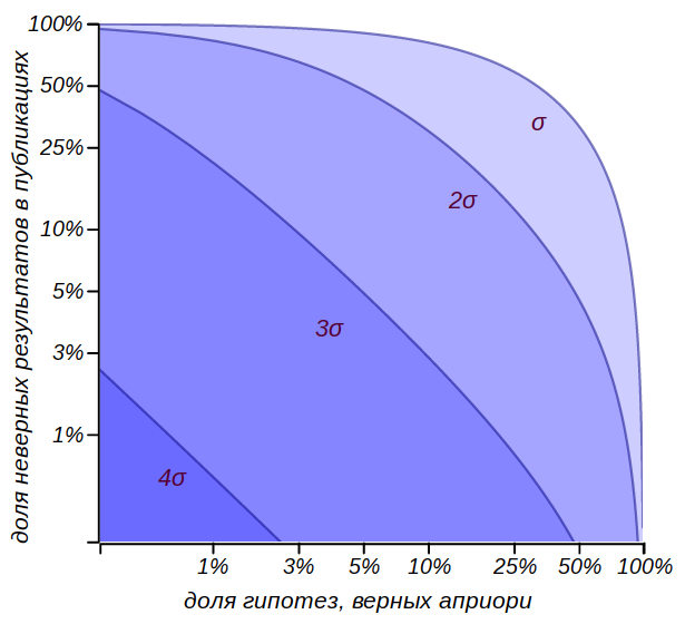
It is easy to get a general estimate of the proportion of incorrect results that will be included in the journal issues, assuming that the proportion of correct hypotheses is equal 0 < α < 1 and the probability of making an erroneous hypothesis isp :
x = ( 1 - α ) pα ( 1 - p ) + ( 1 - α ) p .
Areas that limit the proportion of deliberately incorrect results that can be published in the journal are shown in the figure.
Of course, we don't know that. a l p h a , and we will never know, but it is obviously less than one, which means, in any case, the statement from the editorial column cannot be taken seriously. You can limit yourself to a rigid framework of the criterion. 4 s i g m a , but it requires a very large number of tests. This means that it is necessary to increase the proportion of correct hypotheses in the set of possible assumptions. This is what the standard approaches of the scientific method of knowledge are aimed at - the logical consistency of hypotheses, their consistency with facts and theories that have proved their applicability, reliance on mathematical models and critical thinking.
And again about the weather
At the beginning of the chapter we talked about the fact that weekends and bad weather coincide more often than we would like. Let's try to complete this study. Every rainy day can be viewed as the observation of a random variable — a day of the week that obeys the Bernoulli distribution with probability 1 / 7 . We take as the null hypothesis the assumption that all days of the week are the same in terms of weather and it can rain in any of them equally likely. We have two weekends, in total, we get the expected probability of coincidence of a bad weather day and a holiday equal to 2 / $ , this value will be a parameter of the Bernoulli distribution. How often does it rain? At different times of the year, of course, in different ways, but in Petropavlovsk-Kamchatsky, on average, there are ninety rainy or snowy days per year. So the flow of precipitation days has an intensity of about 90/365 approx1/4 . Let's calculate how many rainy weekends we have to register in order to be sure that there is some pattern. The results are shown in the table.
| Observation period | summer | year | 5 years old |
|---|---|---|---|
| Expected number of observations | 23 | 90 | 456 |
| Expected number of positive outcomes | 6 | 26 | 130 |
| Significant deviation | 4 | 9 | 19 |
| Significant proportion of bad weather in the total number of days off | 42% | 33% | 29% |
What do these numbers say? If it seems to you that that year in a row there was no “summer”, that the evil fate is haunting your weekend, sending rain on them, you can check and confirm it. However, during the summer, evil rock can only be caught if more than two-fifths of the weekend turns out to be rainy. The null hypothesis suggests that only a quarter of the weekend should coincide with inclement weather. For five years of observations, it is already possible to hope to notice subtle deviations beyond the limits of 5% and, if necessary, proceed to their explanation.
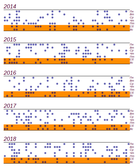
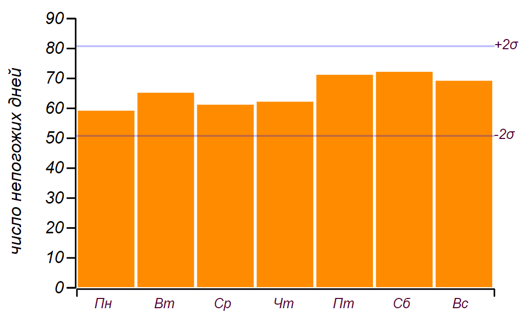
I used the school weather diary, which was conducted from 2014 to 2018, and found out what happened during these five years. 459 rainy days of them 141 come on the weekend. This is indeed more than the expected number on 11 days, but significant deviations begin with 19 days, so this, as we said in childhood: "does not count." This is how the data series and the histogram look, showing the distribution of the weather by days of the week. Horizontal lines on the histogram indicate the interval in which a random deviation from a uniform distribution can be observed with the same amount of data.
The initial data series and the distribution of bad days by days of the week, obtained from five years of observations.
It can be seen that since Friday, there is indeed an increase in the number of days with bad weather. But to find the reason for this growth, the prerequisites are not enough: the same result can be obtained simply by going through random numbers. Conclusion: for five years of weather observation, I have accumulated almost two thousand records, but I did not learn anything new about the distribution of weather by days of the week.
When looking at the diary entries, it is clearly striking that bad weather does not come one by one, but two or three-day periods, or even weekly cyclones. Does it somehow affect the result? You can try to take this observation into account, and assume that it rains an average of two days (in fact, 1.7 days), then the probability to cut off the weekend increases to 3/7 . With such a probability, the expected number of matches for five years should be 195 pm21 that is from 174 before 216 time. Observed value 141 does not fall within this range, which means that the hypothesis of the effect of double weather days can be safely rejected. Did we learn something new? Yes, we learned: it would seem that the obvious feature of the process does not entail any effect. This is worth considering, and we will do it a little later. But the main conclusion: there are no reasons to consider any more subtle effects, since observations and, most importantly, their number, consistently speak in favor of the simplest explanation.
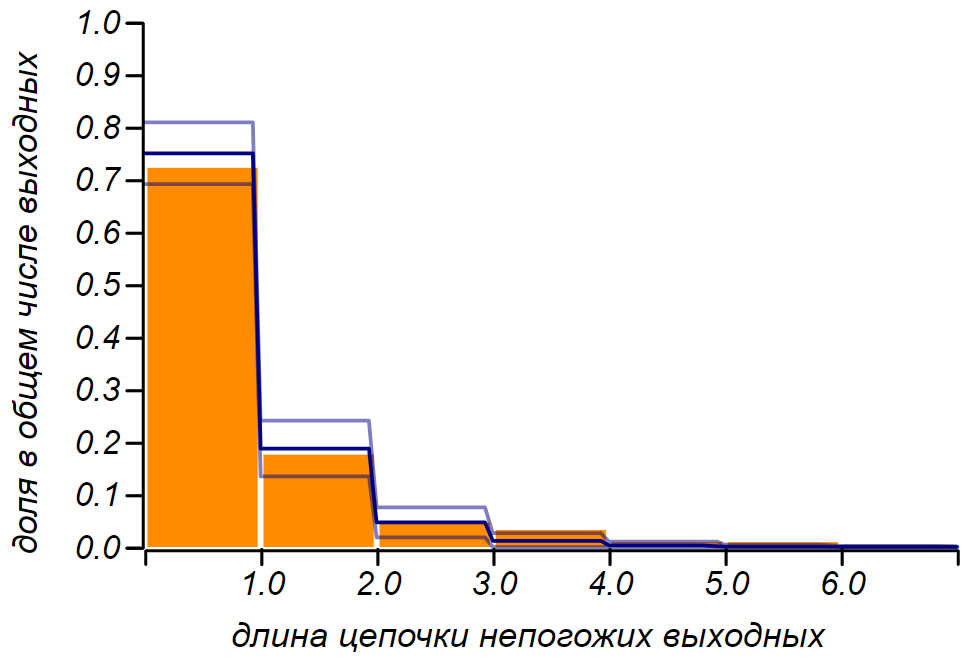
But our discontent is caused not by five-year or even annual statistics, human memory is not so long. It's a shame when it rains over the weekend three or four times in a row! How often can this be observed? Especially if you remember that the nasty weather does not come alone. The task can be formulated as: "What is the probability that n Weekend in a row will be rainy? ”It is reasonable to assume that bad days form a Poisson stream with intensity 1/4 . This means that, on average, a quarter of the days of any period will be bad weather. Observing only the weekends, we should not change the intensity of the flow and from all the weekends the bad weather should make up, on average, also a quarter. So, we put forward the null hypothesis: the Poisson flow of bad weather, with a known parameter, and therefore, the intervals between Poisson events are described by an exponential distribution. We are interested in discrete intervals: 0, 1, 2, 3 of the day, etc., so we can use the discrete analogue of the exponential distribution — the geometric distribution with the parameter 1/4 . The figure shows that we have succeeded and it is clear that the assumption that we are observing the Poisson process has no reason to reject.
The observed distribution of the lengths of the failed output chains is theoretical. The thin line shows the tolerances for the number of observations that we have.
One may ask, such a question: how many years it is necessary to conduct observations, in order that we notice the difference in 11 days could you confidently confirm or reject as random rejection? It is easy to calculate: the observed probability 141/459=$0.30 different from expected 2/7=0.286 on 0.02 . To fix the difference in hundredths, an absolute error is required, not exceeding 0.005 , what is 1.75% from the measured value. From here we obtain the required sample size. n geq(4 cdot5/7)/(0.01752 cdot2/7) approx$3200 rainy days. It will take about 4 cdot32000/365 approx360 years of continuous meteorological observations, because only every fourth day it rains or snows. Alas, this is more than the time that Kamchatka is in Russia, so I have no chance to find out how things are “in fact”. Especially if we take into account that during this time the climate has changed dramatically - from the Little Ice Age, nature emerged at the next optimum.
So how did Australian researchers manage to fix the deviation of temperature in a fraction of a degree, and why does it make sense to consider this study? The fact is that they used hourly temperature data that was not “thinned out” by any random process. So for 30 years of meteorological observations, it was possible to accumulate more than a quarter of a million counts, which makes it possible to reduce the standard deviation of the average 500 times relative to standard daily temperature deviation. This is quite enough to talk about accuracy in tenths of a degree. In addition, the authors used another beautiful method confirming the existence of a time cycle: random mixing of the time series. Such mixing preserves statistical properties, such as flow intensity, but “erases” temporal patterns, making the process truly Poisson. Comparison of the set of synthetic series and the experimental one makes sure that the observed deviations from the Poisson process are significant. In the same way, the seismologist A. A. Gusev showed that earthquakes in an area form a kind of self-similar flow with clustering properties. This means that earthquakes tend to cluster in time, forming a very unpleasant stream seals. Later it turned out that the sequence of large volcanic eruptions has the same property.
Another source of chance
Of course, the weather, like earthquakes, cannot be described by the Poisson process - these are dynamic processes in which the current state is a function of the previous ones. Why do our weekend weather observations speak in favor of a simple stochastic model? The fact is that we map the regular process of precipitation formation to a set of seven days, or, speaking in the language of mathematics, to a system of residues modulo seven . This projection process is capable of generating chaos from well-ordered data series. Hence, for example, there is a visible randomness in the sequence of digits of the decimal notation of the majority of real numbers.
We have already spoken about rational numbers, those that are expressed as integer fractions. They have an internal structure, which is determined by two numbers: the numerator and the denominator. But when writing in decimal form, one can observe jumps from regularity in the representation of such numbers as 1/2=0.5 overline0 , or 1/3=0. Overline3 until periodic repetition, already completely disordered sequences in such numbers as 1/17=0. Overline0588235294117647 . Irrational numbers do not have a finite or periodic record in decimal form, and in this case chaos reigns in the sequence of numbers. But this does not mean that there is no order in these numbers! For example, the first irrational number met by mathematicians sqrt2 in decimal notation generates a chaotic set of numbers. However, on the other hand, this number can be represented as an infinite continued fraction:
sqrt2=1+ frac12+ frac12+ frac12+....
It is easy to show that this chain is really equal to the root of two, having solved the equation:
x−1= frac12+(x−1).
Continued fractions with repeating coefficients are written briefly, like periodic decimal fractions, for example: sqrt2=[1, bar2] , sqrt3=[1, overline1,2] . The famous golden section in this sense is the simplest arranged irrational number: varphi=[1, bar1] . All rational numbers are represented as finite continued fractions, some irrational - as infinite, but periodic, they are called algebraic , the same that do not have a finite notation even in this form - transcendental . The most famous of the transcendental is the number pi it creates chaos both in decimal notation and in the form of a continued fraction: pi approx[3,7,15,1,292,1,1,1,1,1,1,3,1,14,2,1,...] . But the Euler number e while remaining transcendental, in the form of a continued fraction, it exhibits an internal structure hidden in the decimal notation: e approx[2,1,2,1,1,4,1,1,6,1,1,8,1,1,10,...] .
Probably not one mathematician, starting with Pythagoras, suspected the world of cunning, discovering what is necessary, such a fundamental number pi has such an elusively complex chaotic structure. Of course, it can be presented in the form of sums of quite elegant numerical series, but these series do not directly speak about the nature of this number and they are not universal. I believe that the mathematicians of the future will open up some new representation of numbers, as universal as continued fractions, which will reveal the strict order hidden by nature in the number.
∗ ∗ ∗
The results of this chapter are, for the most part, negative. And as an author who wants to surprise the reader with hidden patterns and unexpected discoveries, I wondered whether to include it in a book. But our conversation about the weather went into a very important topic - about the value and meaningfulness of the natural science approach.
One wise girl, Sonya Shatalova, looking at the world through the prism of autism, at the age of ten gave a very concise and precise definition: “Science is a system of knowledge based on doubt . ” The real world is unsteady and strives to hide behind the complexity, apparent randomness and unreliability of measurements. Doubt in the natural sciences is inevitable. Mathematics seems to be the realm of certainty, in which, it seems, you can forget about doubt. And it is very tempting to hide behind the walls of this kingdom; consider instead of the difficult to recognize world models that can be thoroughly investigated; read and calculate, the benefit of the formula ready to digest anything. But nevertheless, mathematics is a science and doubt in it is a deep inner honesty, which does not give rest until the mathematical construction is cleared of additional assumptions and unnecessary hypotheses. In the realm of mathematics, they speak a complex but well-proportioned language suitable for reasoning about the real world. It is very important to get acquainted with this language a little, in order not to let the numbers impersonate statistics, not to let the facts pretend to be knowledge, but to oppose real science to ignorance and manipulation.
Source: https://habr.com/ru/post/435812/
All Articles