Forecasting again, part 1

Consider the prediction of time series. Let us try to predict the charts of quotations, or something else that comes to hand.



Let us take as a basis the forecasting presented in the article The Time Series Prediction Model for a Sample of Maximum Similarity: an explanation and an example (this article is not mine). The brief point is that the most similar segment of the graph to the left of the forecast is searched for among past history, and from this old best, then the values ​​to the right of the graph are taken and used as a forecast.

I will go on. When calculating the forecast, I will take not one best case by correlation, but a pack of the best ones. And the forecast will be the average of the results for this pack. This will make it possible to understand that the value found is a regularity, and not a random coincidence with the desired forecast, or a random deviation, if the forecast deviates from the actual.
')
Using the single best case as in that article is not correct, as well as determining the probability distribution by a single value from this distribution. If you generate a very large graph of random data, and run a search on them, then there will necessarily be correlated segments, and it is even possible with a coefficient of 0.9999, but it is not at all necessary that such continuations will continue to follow these segments - it is still all randomly. And you need to take exactly a pack of such segments and calculate that the variance of the subsequent data is lower than the variance that is formed from a random sample of this data. And if the dispersion of the packet is lower, then this is a forecast. Although this is not the same exact representation of possible errors, but so far this is enough.

Those. forecasting is not what principle of sampling and correlation of the compared segments we use, the main thing is that as a result of applying this sample, the variance of the desired values ​​would be less than as a result of random sampling.

Also the dispersion of this pack will give the opportunity to evaluate which is better to use the selection option among previous cases. After all, it is not always possible to select a segment of correlated data one by one, and not always use the Pearson correlation. And such a choice can be made for each predicted point separately. For what type of sample the variance is less, that option is better for the current point.

What is the size of the pack should be? This rests on the question of confidence intervals. That would not be very loaded, there is a mention that to determine the average value is better to take at least 30 examples. If there is an excess of test data, I would take at least 100.

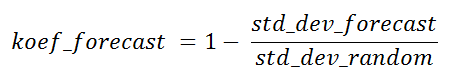
The ratio of the standard deviations of the sample according to the algorithm and the sample randomly can be called the theoretical success rate of the prediction algorithm for the current point for comparison purposes with other sampling algorithms, or for determining the utility of this forecast at all, while the actual value itself is not yet available.



This coefficient may in some cases take on negative values. The points at which this occurs are of little interest, as are the points with zero coefficient. In the case of 100% predictability, it will be equal to one.

Let us turn to practical examples, again from that article. After correcting the minor bugs there, we get the following result:

calculation of the forecast at the time of 9/1/2012 23:00 position 52631
total values ​​tested for similarity 2184
the best correlation is 0.958174 position 52295
transfer coefficients alpha (1/2) 1.03117 -11.1992
forecast error from mape fact 5.210%

mape - a term from the original article Mean Absolute Percentage Error, is calculated by the formula
Abs (Forecast - Fact) / Fact

And now let's make a sample of not one best similarity, but packs of the best and all for predicting one moment in time and see what happens:

0 corr 0.958174 pos 52295 mape 5.210%
1 corr 0.953571 pos 52151 mape 6.566%
2 corr 0.953532 pos 45599 mape 11.642%
3 corr 0.951462 pos 45743 mape 7.033%
4 corr 0.950921 pos 45575 mape 3.300%
5 corr 0.950789 pos 38687 mape 3.538%

The correlation value here varies from value to value negligible. At the same time, the value of the forecast result varies from 3% to 11%. Those. those initial 5% are nothing but an accident, it could be 11% and 3%.

Under the conditions specified in that article, a sample of similarity can be compared with a total of 2184 values. Of these, I took the best pack of 1500 pieces, sorted in order of decreasing correlation, and displayed it as a graph. The correlation in this pack from the best 0.958 dropped to 0.715 from left to right. But the fluctuation of the result practically did not change:



It can be seen that the dependence of the result on the correlation is very low, but nevertheless it seems to be there. In general, take a pack of the top 100 values, and calculate the forecast, as I mentioned, by the average for this pack. The result is the following: mape 5.824%, stddev mape 7.035% . But this 5.8% is no longer a coincidence, but the average of the distribution is the most likely forecast. The standard deviation of a mape exceeds the mape itself, but this is because the mape has a non-symmetrical distribution.

I also calculated the same forecast, but for a conditionally random sample, or rather, just averaged from all possible options, the result of mape is 8.246% . For a random sample, the error is slightly larger, but this value is still within the range of the variation that was calculated from the best sample. For the calculated point, the theoretical prediction coefficient indicated by me is close to zero, more precisely, koef_forecast = -0.041 . I considered it not from the stddev mape (it includes the actual forecast), but from the absolute values ​​of the forecast, if you watch the program, then the original figures for it are given there.

But this is if regarding the timestamp, which was mentioned in the original article. But if we take, say, “9/4/2012 23:00” (month / day / year time), then there the theoretical utility coefficient is koef_forecast = 0.21 , and mape = 3.126%, mape_rand = 7.147% . Those. koef_forecast showed in advance that the current point will be calculated more accurately than the previous one. The essence of the utility of this coefficient is that you can somehow evaluate the result before obtaining the actual data, because no actual data is involved. The higher it is, the better. I have already mentioned that an absolutely predictable point will have a factor of one.

You yourself can see how all these numbers change in my demo program on Qt C ++, there you can choose both the date and the size of the pack: source code on github

The selection of the best values ​​is made according to the following algorithm:

inline void OrdPack::add_value(double koef, int i_pos) { if (std::isfinite(koef)==false) return; if (koef <= 0.0) return; if (mmap_ord.size() < ma_count_for_pack) { if (mmap_ord.size()==0) mi_koef = koef; mi_koef = std::min(mi_koef, koef); mmap_ord.insert({-koef,i_pos}); } else if (koef > mi_koef) { mmap_ord.insert({-koef,i_pos}); while (mmap_ord.size() > ma_count_for_pack) mmap_ord.erase(--mmap_ord.end()); mi_koef = -(--mmap_ord.end())->first; } } 

The point here is to post the entire source is not, there it is not complicated, and with comments. The basis of the MainWindow :: to_do_test () procedure in the mainwindow.cpp file.

For now, I’ll continue to try to predict something in the next part.

Ps. Please leave your comments on whether everything is clear about what is missing. I have already formed an approximate plan, what to write next, but with your comments, I will do it better.