NeurIPS-2018 Review (ex. NIPS)
In early December, the 32nd annual Neural Information Processing Systems conference was held in Montreal, dedicated to machine learning. According to the unofficial table of ranks, this conference is the top-1 event of a similar format in the world. All conference tickets this year were sold out in a record 13 minutes. We have a large data scientist team of MTS, but only one of them - Marina Yaroslavtseva ( magoli ) - was lucky enough to get to Montreal. Together with Danila Savenkov ( danila_savenkov ), who was left without a visa and followed the conference from Moscow, we will tell you about the works that we found most interesting. This sample is very subjective, but we hope it will interest you.

Relational recurrent neural networks
Abstract
Code
')
When working with sequences it is often very important how the elements of a sequence are related to each other. Standard recurrent network architectures (GRU, LSTM) can hardly model the relationship between two elements that are sufficiently distant from each other. To some extent, attention ( https://youtu.be/SysgYptB198 , https://youtu.be/quoGRI-1l0A ) helps to cope with this, but still it is not quite that. Attention allows you to determine the weight with which the hidden state from each of the steps in the sequence will affect the final hidden state and, accordingly, the prediction. We are interested in the interrelation of the elements of the sequence.
Last year, again on the NIPS, google suggested to completely abandon recurrence and use self-attention . The approach proved to be very good, though mostly on seq2seq tasks (the article presents the results of machine translation).
The authors of this year’s article use the idea of self-attention as part of LSTM. There are not many changes:
It is argued that it is through MHDPA that the grid can take into account the interrelation of the elements of the sequence even when they are separated from each other.
As a toy problem, the model is asked to find the Nth vector in the sequence of vectors by the distance from the Mth in terms of the Euclidean distance. For example, there is a sequence of 10 vectors and we ask to find one that is in third place in proximity to the fifth. It is clear that to answer this question, the model needs to somehow estimate the distances from all the vectors to the fifth and sort them. Here, the model proposed by the authors confidently wins LSTM and DNC . In addition, the authors compare their model with other architectures at the Learning to Execute (we receive several lines of code as input, issue the result), Mini-Pacman, Language Modeling, and everywhere report on the best results.
Multivariate Time Series Imputation with Generative Adversarial Networks
Abstract
Code (although the article does not link here)
In multidimensional time series, as a rule, there are a large number of gaps, which hinders the use of advanced statistical methods. Standard solutions - filling with the middle / zero, removing incomplete cases, recovering data based on matrix expansions in this situation often do not work, because they cannot reproduce the time dependencies and the complex distribution of multidimensional time series.
The ability of generative-adversary networks (GANs) to imitate any distribution of data, in particular, in the tasks of “drawing” persons and generating sentences, is widely known. But, as a rule, such models either require initial training in full dataset without gaps, or do not take into account the consistent nature of the data.
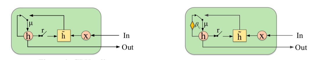
The authors propose to supplement GAN with a new element - the Gated Recurrent Unit for Imputation (GRUI). The main difference from the usual GRU is that GRUI can be trained on data with intervals of different lengths between observations and correct the influence of observations depending on their distance in time from the current point. A special attenuation parameter β is calculated, the value of which varies from 0 to 1 and the smaller, the longer the time lag between the current observation and the previous non-empty one.

Both the discriminator and the GAN generator consist of a GRUI layer and a fully connected layer. As usual in the GANs, the generator learns to imitate the original data (in this case, just fill in the gaps in the rows), and the discriminator learns to distinguish the rows filled with the generator from the real ones.
As it turned out, such an approach very adequately recovers data even in time series with a very large proportion of gaps (in the table below - MSE data recovery in the KDD data, depending on the fraction of gaps and recovery method. In most cases, the GAN-based method gives the greatest accuracy recovery).
On the Dimensionality of Word Embeddings
Abstract
Code
Word embedding / vector word representation is an approach widely used for various NLP applications: from recommender systems to analyzing the emotional coloring of texts and machine translation.
At the same time, the question of how to optimally set such an important hyperparameter as the dimension of vectors remains open. In practice, it is most often selected by empirical brute force or set by default, for example, at the level of 300. At the same time, too small dimension does not reflect all significant interrelationships between words, and too large can lead to retraining.
The authors of the study propose their solution to this problem by minimizing the PIP loss parameter, a new measure of the difference between the two embedding options.
The calculation is based on PIP-matrices, which contain the scalar products of all pairs of vector representations of words in the body. PIP loss is calculated as the Frobenius norm between the PIP-matrices of two embeddings: trained on data (trained embedding E_hat) and perfect, trained on non-noisy data (oracle embedding E).
It would seem that everything is simple: you need to choose a dimension that minimizes PIP loss, the only incomprehensible point is where to get the oracle embedding. In 2015-2017, a number of papers were published in which it was shown that various methods for constructing embeddings (word2vec, GloVe, LSA) implicitly factorize (lower the dimension) the signal matrix of the case. In the case of word2vec (skip-gram), the signal matrix is PMI , in the case of GloVe, the log-counts matrix. It is proposed to take a dictionary of very large size, build a signal matrix and use SVD to obtain oracle embedding. Thus, the dimension of oracle embedding is obtained equal to the rank of the signal matrix (in practice, for a dictionary of 10k words, the dimension will be about 2k). However, our empirical signal matrix is always noisy and we have to resort to clever schemes to get oracle embedding and evaluate the PIP loss using a noisy matrix.
The authors argue that to select the optimal embedding dimension it is enough to use a dictionary of 10k words, which is not very much and allows you to get rid of this procedure in a reasonable time.
As it turned out, the embedding dimension thus calculated in most cases with an error of up to 5% coincides with the optimal dimension, determined on the basis of expert estimates. It turned out (expectedly) that Word2Vec and GloVe practically do not retrain (PIP loss on very large dimensions does not fall), but LSA retrains quite strongly.
With the help of the code laid out by the authors, you can search for the optimal dimension of Word2Vec (skip-gram), GloVe, LSA.
FRAGE: Frequency-Agnostic Word Representation
Abstract
Code
The authors talk about how embeddingings work differently for rare and for popular words. By popular, I mean not stop words (we don’t consider them at all), but meaningful words that are not very rare.
The observations are as follows:
If we talk about popular words, then their proximity is cosine very well reflected.
Whatever the case with the ratio of embeddingd L2-norms, the separability of popular and rare words is not a very good phenomenon. We want the embeddings to reflect the semantics of the word, not its frequency.
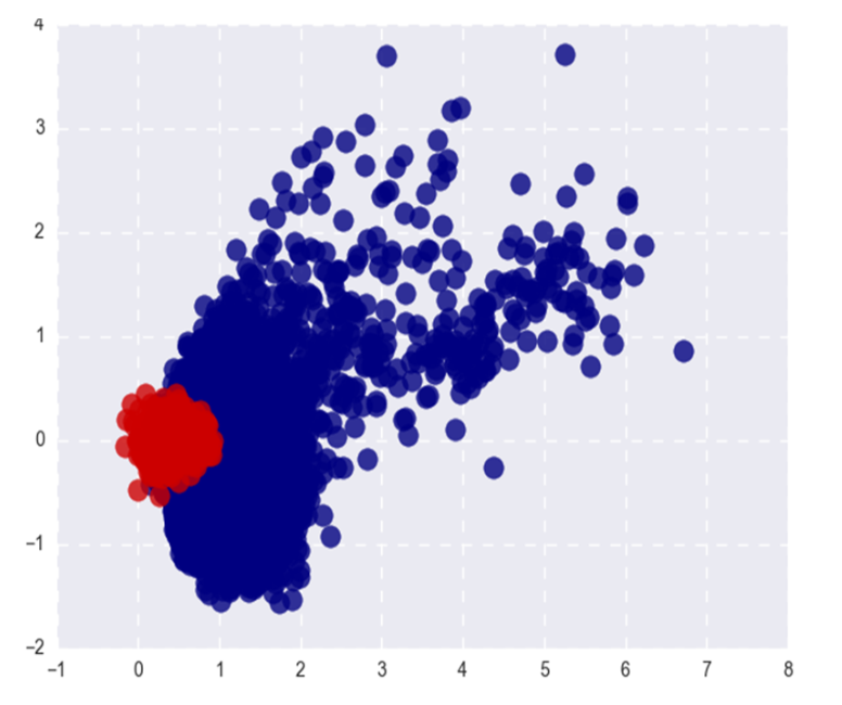
The picture shows popular Word2Vec (red) and rare (blue) words after SVD. Under popular here refers to the top 20% of the words in frequency.
If the problem was only in the L2-norms of embeddings, we could normalize them and live happily, but, as I said in the first paragraph, in cosine proximity (in polar coordinates) rare words are also separated from popular ones.
The authors propose, of course, the GAN. Let's do everything the same as before, but add a discriminator that will try to distinguish popular words from rare ones (again, we consider the top n% words in frequency to be popular).
It looks like this:
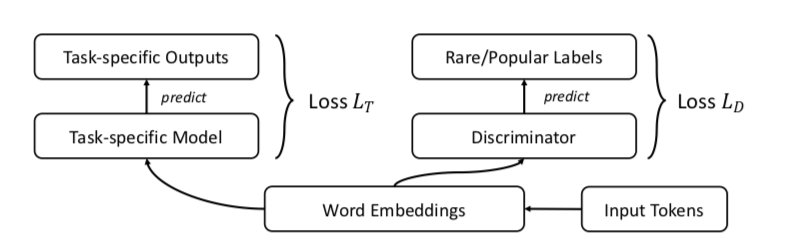
The authors test the approach on the tasks of word similarity, machine translation, text classification and language modeling and everywhere perform better baseline. In word similarity it is argued that quality grows especially noticeably in rare words.
One example: citizenship. Skip-gram issues: bliss, pakistans, dismiss, reinforces. FRAGE issues: population, städtischen, dignity, bürger. The words citizen and citizens at FRAGE at 79 and 7 place, respectively (in proximity to the citizenship), at skip-gram - are not in the top 10000.
For some reason, the authors posted the code only for the tasks of machine translation and language modeling, word similarity and text classification in the repository, unfortunately, are not represented.
Unsupervised Cross-Modal Alignment of Speech and Text Embedding Spaces
Abstract
Code: no code, but I would like to
Recent studies have shown that two vector spaces, trained using embedding algorithms (for example, word2vec) on text boxes in two different languages, can be matched to each other without marking and matching the contents of the two bodies to each other. In particular, this approach is used for machine translation in the company Facebook. One of the key properties of embedding spaces is used: inside them, similar words must be geometrically close, and unlike - on the contrary, be far from each other. It is assumed that, in general, the structure of the vector space is preserved regardless of the language in which the corpus was used for learning.
The authors of the article went further and applied a similar approach to the field of automatic speech recognition and translation. It is proposed to teach the vector space separately for the text corpus in the language of interest (for example, Wikipedia), separately for the corpus of recorded speech (in audio format), perhaps in another language, previously broken into words, and then to compare these two spaces similarly to the two text enclosures.
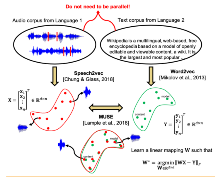
For text body, word2vec is used, and for speech, a similar approach, called Speech2vec, based on LSTM and methodologies used for word2vec (CBOW / skip-gram), so it is assumed that it combines words according to contextual and semantic characteristics, and not sounding.
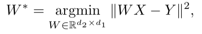
After both vector spaces are trained and there are two sets of embeddings - S (on the body of speech), consisting of n embeddings of dimension d1 and T (on the body of text), consisting of m embeddings of dimension d2, you need to match them. Ideally, we have a dictionary that determines which vector from S corresponds to which vector from T. Then two matrices are formed for comparison: from S we choose k embeddings that form a matrix X of size d1 xk; from T, too, k embeds are chosen that correspond (in the dictionary) to those previously selected from S, and a matrix Y of size d2 x k is obtained. Next, you need to find a linear mapping W such that:
But since the article discusses the unsupervised approach, there is initially no dictionary, so the procedure for generating a synthetic dictionary, consisting of two parts, is proposed. First, we get the first approximation of W using the domain-adversarial training (competitive model like GAN, only instead of the generator - linear display W, with which we try to make S and T indistinguishable from each other, and the discriminator tries to determine the real origin of embedding). Then, based on the words, the embeddingings of which showed the best fit to each other and are most often found in both cases, a dictionary is formed. After this, W is refined according to the formula above.
This approach gives results comparable to learning on labeled data, which can be very useful in the problem of speech recognition and translation from rare languages for which there are too few parallel speech-text shells, or they are missing.
Deep Anomaly Detection Using Geometric Transformations
Abstract
Code
An unusual approach to anomaly detection, which, according to the authors, greatly overcomes other approaches.
The idea is this: let's invent K different geometric transformations (combinations of shifts, rotate 90 degrees and reflections) and apply them to each picture of the original dataset. The picture resulting from the i-th transformation will now belong to class i, that is, there will be K classes in total, each of them will be represented by such a number of pictures that was originally in dataset. Now we will teach a multi-class classification on such markup (the authors chose wide resnet).
Now we can get K vectors y (Ti (x)) of dimension K, where Ti is the i-th transformation, x is the picture, y is the output of the model. The basic definition of “normality” is as follows:
Here, for the image x, we add the predicted probabilities of the correct classes for all transformations. The greater the “normality”, the more likely it is that the image is taken from the same distribution as the training sample. The authors claim that it already works very well, but nevertheless they offer a more complex way that works even better. We will assume that the vector y (Ti (x)) for each transformation Ti is distributed over Dirichlet and as a measure of the “normality” of the image we will consider the log likelihood. The Dirichlet distribution parameters are estimated on the training set.
The authors report an incredible boost of performance compared to other approaches.
A Simple Unified Framework for Detecting Out of Distribution and Adversarial Attacks
Abstract
Code
Identifying cases in a sample for applying a model that is significantly different from the distribution of a training sample is one of the basic requirements for obtaining reliable classification results. At the same time, neural networks are known for their feature with a high degree of certainty (and incorrectly) to classify objects that have not been encountered in training, or that are intentionally destructive (adversarial examples).
The authors of the article propose a new method of identifying both those and other "bad" cases. The approach is implemented as follows: first, the neural network is trained with the usual softmax output, then the output of its penultimate layer is taken, and the generative classifier is trained on it. Let there be x - what is fed to the input of the model for a specific classification object, y is the corresponding class label, then suppose that we have a pre-trained softmax classifier of the form:
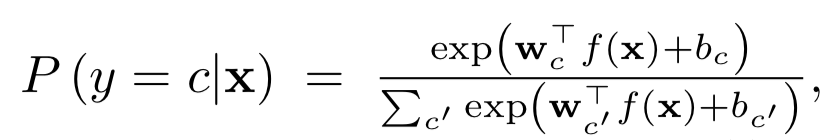
Where wc and bc are weights and softmax layer constant for class c, and f (.) Is the output of the last but one soybean DNN.
Further, without any changes to the pre-trained classifier, a transition is made to the generative classifier, namely discriminant analysis. It is assumed that the signs taken from the penultimate layer of the softmax classifier have a multidimensional normal distribution, each component of which corresponds to one class. Then the conditional distribution can be defined through the vector of averages of the multidimensional distribution and its covariance matrix:

To estimate the parameters of the generative classifier, empirical averages are calculated for each class, as well as the covariance for cases from the training set {(x1, y1), ..., (xN, yN)}:
where N is the number of cases of the corresponding class in the training sample. Then, on the test sample, a measure of reliability is calculated - the Mahalanobis distance between the test case and the normal distribution of the class closest to this case.
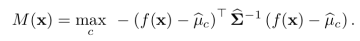
As it turned out, such a metric works much more reliably on atypical or spoiled objects, without giving overestimated estimates, as in the softmax layer. In most comparisons on different data, the proposed method showed results that exceeded the current state-of-the-art in finding both cases that were not in training, and intentionally spoiled.
Next, the authors consider another interesting application of their methodology: use the generative classifier to highlight new classes on the test, which were not in training, and then update the parameters of the classifier itself so that it can later determine this new class.
Adversarial Examples that Fool both Computer Vision and Time-Limited Humans
Abstract: https://arxiv.org/abs/1802.08195
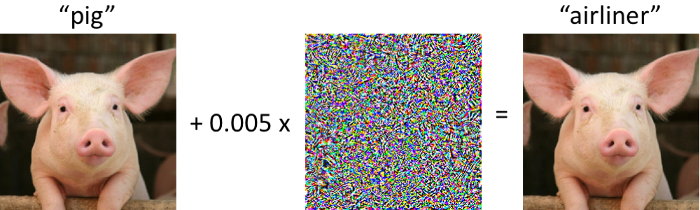
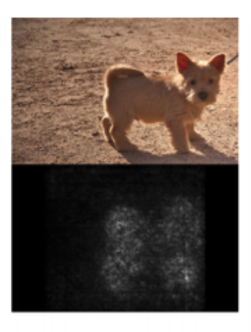
The authors investigate what adversarial examples are from the point of view of human perception. Today, no one is surprised by the fact that it is possible almost without changing the image to make the network make mistakes on it. However, it is not very clear how the original picture differs from the adversarial example for a person and if it differs at all. It is clear that none of the people will call the picture on the right an ostrich, but still, perhaps the picture on the right for a person is not exactly identical to the picture on the left, and, if so, a person can also be exposed to adversarial attacks.
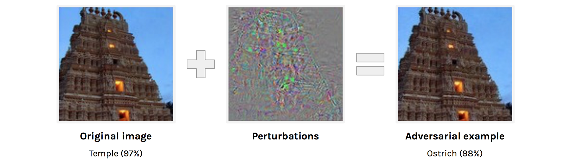
The authors try to assess how well a person can classify adversarial examples. To obtain adversarial examples, a technique is used which does not have access to the architecture of the original network (the authors' logic is that they still will not be given access to the architecture of the human brain).
So, a person is shown adversarial example, as in the picture above and asked to classify it. It is clear that in normal conditions the result would be predictable, but here one image is shown to a person for 63 milliseconds after which he must choose one of two classes. In such conditions, the accuracy of the original images was 10% higher than the adversarial. In principle, this could be explained by the fact that the adversarial image is simply noisy and therefore, in the conditions of a shortage of time, people incorrectly classify it, but this refutes the following experiment. If, before adding perturbation to the image, we reflect this perturbation vertically, then accuracy will hardly change compared to the original image.
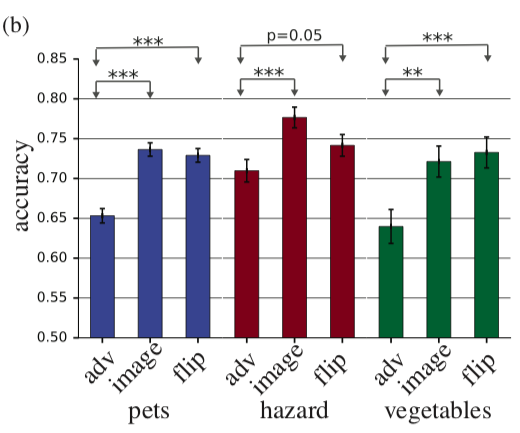
On the histogram adv - adversarial example, image - the original image, flip - the original image + adversarial perturbation, reflected vertically.
Sanity Checks for Saliency Maps
Abstract
Interpretation of models is one of the most discussed topics today. If we are talking about deep learning, we usually talk about saliency maps. Saliency maps try to answer the question of how the value changes at one of the grid outputs when the input values change. This may look like a saliency map, which shows which pixels affected the image being classified as a “dog”.
The authors ask a very reasonable question: “How would we validate the methods of constructing saliency maps?” Two obvious theses are put forward that are proposed to be tested:
We will check the first thesis, replacing the weights in the trained grid with randomization: cascading randomization (random layers, starting with the last one and see how the saliency map changes) and independent randomization (random random layers). The second thesis will be checked like this: randomly we mix all the labels on the train, overfit the train and look at the saliency maps.
If the method of constructing a saliency map is really good and allows you to understand how the model works, such randomization should greatly change the saliency maps. However: “To our surprise, some widely deployed,” the authors state. Here, for example, how saliency maps, obtained using various algorithms, after cascading randomization look like:
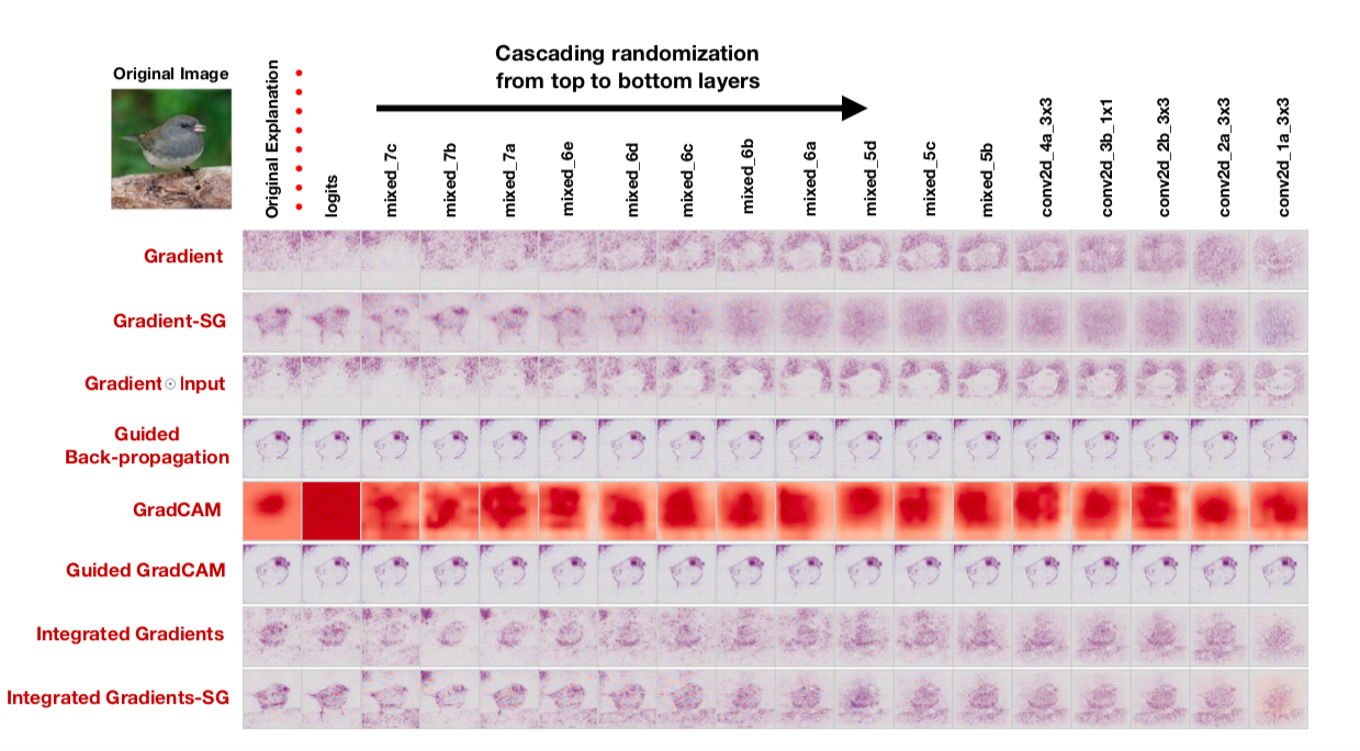
Note the funny fact that the last column corresponds to a grid with random weights in all layers. That is, the grid predicts randomly, but some saliency maps still draw a bird.
The authors rightly say that - assessment of saliency maps by their comprehensibility and consistency and insufficient attention to the extent to which the result is related to how the model works leads to a confirmation bias. Apparently, including for this reason, it turns out that common approaches to the interpretation of models do not interpret them at all.
An intriguing failing of convolutional neural networks and the CoordConv solution
Abstract: https://arxiv.org/abs/1807.03247
Code: there are already many implementations, and in general the idea is so beautiful and simple that it is written literally in 10 lines.
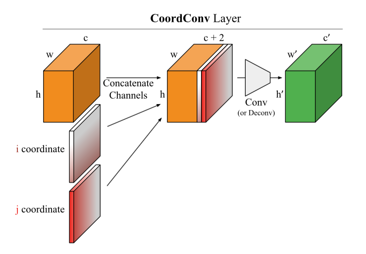
A simple and promising idea from Uber. Convolutional networks are initially sharpened for shear invariance, so the tasks associated with determining the coordinates of an object for such networks are very difficult. Ordinary convolutional networks are not able to solve even toy problems such as determining the coordinates of a point in a picture or drawing a point along coordinates:
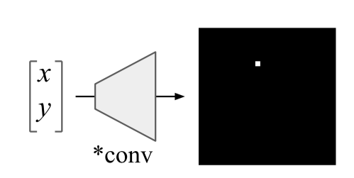
A very elegant hack is proposed: add to the picture (in general, to the CoodrConv layer input) two matrices i and j, which will contain the vertical and horizontal coordinates of the corresponding pixels:
It is alleged that:
Personally, the second point is more interesting to me from this, I would like to see the results on real datasets, but at the same time nothing is googled. Meanwhile, CoordConv is already actively building in U-net : https://arxiv.org/abs/1812.01429, https://www.kaggle.com/c/tgs-salt-identification-challenge/discussion/69274 , https: //github.com/mjDelta/Kaggle-RSNA-Pneumonia-Detection-Challenge .
There is a good and more detailed video from the author .
Regularizing by the Variance of the Activations' Sample-Variances
Abstract
Code
The authors offer a fun alternative to batch normalization. We will fine the grid for the variability of the dispersion of activations on some layer. : S1 S2 :
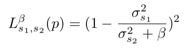
σ2 — S1 S2 , β — . variance constancy loss (VCL) .
, (). 11- (CIFAR-10 CIFAR-100). , VCL , Leaky ReLU ELU, ReLU batch normalization. 2 Tiny Imagenet — Imagenet 200 64x64. VCL batch normalization ELU, ResNet-110 DenseNet-40, Wide-ResNet-32. , , S1 S2 .
VCL feed-forward VCL , batch normalization .
DropMax: Adaptive Variational Softmax
Abstract
- . , , . , “” , .
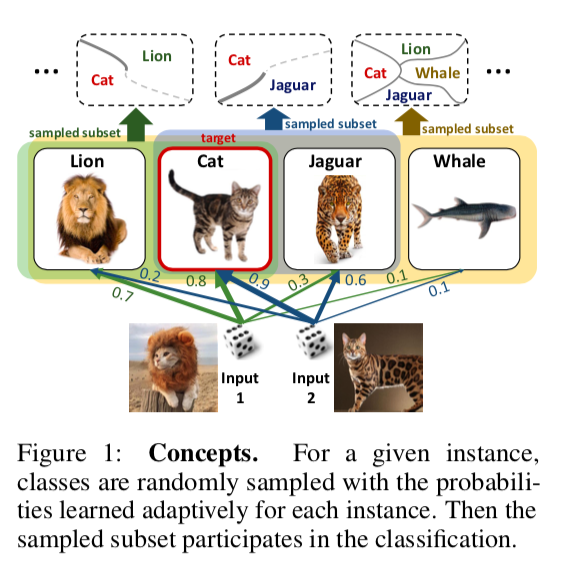
MNIST, CIFAR Imagenet , DropMax SoftMax, .
Accurate Intelligible Models with Pairwise Interactions
(Friends Don't Let Friends Deploy Black-Box Models: The Importance of Intelligibility in Machine Learning)
Abstract: http://www.cs.cornell.edu/~yinlou/papers/lou-kdd13.pdf
: . , . , =)
, : https://github.com/dswah/pyGAM . feature interactions ( GAM GA2M).
“Interpretability and Robustness in Audio, Speech, and Language”, , ., - . , , . « », , , , , , . , , , - , . .

, : . : , , . , , , . xgboost , , , , , .
, , — GA2M, (Generalized additive models).
GAM , GLM: , , , GLM, ( , – , «»). GAM , . , () .
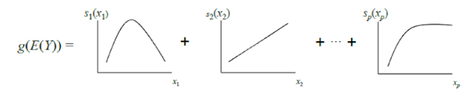
GAM « ». , – , , – , . GA2M.
GAM ( ), ( GAM). , , FAST, .
, . , GA2M c FAST .
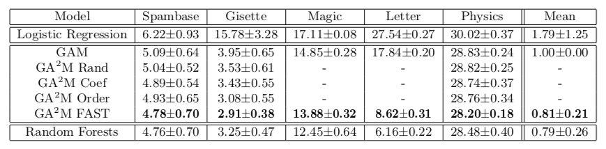
, . , , 20 ( UCI). : 2018 . 50 — , .
— . . , , , , — black-box . , , , .
, . . 10 ( L2- ), , , predict_proba 0.86. , sparse . , L1-, . L1- . 0, , , . , . , interpretable and credible models .
Visualization for Machine Learning: UMAP
Absract
“Visualization for Machine Learning” Google Brain. , , , , , – , , , .., . , .
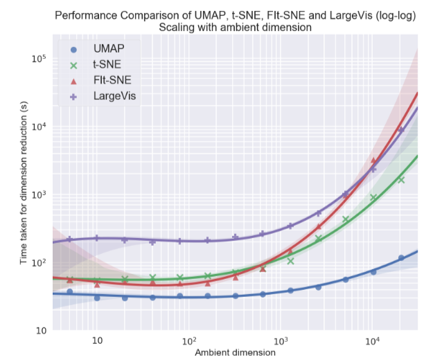
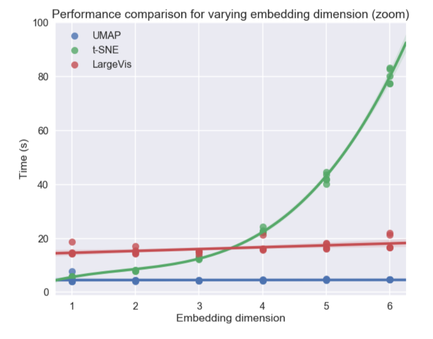
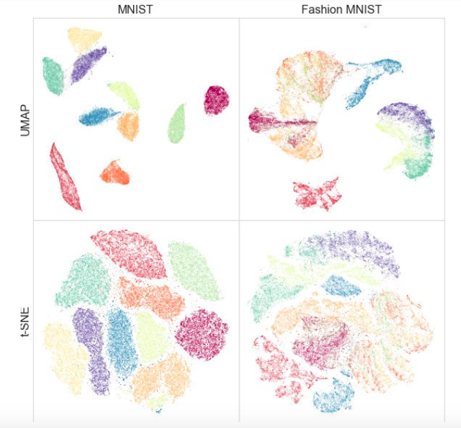
, Uniform Manifold Approximation and Projection (UMAP) – . , , , . , UMAP t-SNE 2-10 , , :
, t-SNE UMAP , (. . ), ( ) — , .
, UMAP , t-SNE: , MNIST Fashion MNIST UMAP:
— : UMAP sklearn, sklearn pipeline. , , UMAP , t-SNE, .. .
semi-supervised — , UMAP .
? , , .
Relational recurrent neural networks
Abstract
Code
')
When working with sequences it is often very important how the elements of a sequence are related to each other. Standard recurrent network architectures (GRU, LSTM) can hardly model the relationship between two elements that are sufficiently distant from each other. To some extent, attention ( https://youtu.be/SysgYptB198 , https://youtu.be/quoGRI-1l0A ) helps to cope with this, but still it is not quite that. Attention allows you to determine the weight with which the hidden state from each of the steps in the sequence will affect the final hidden state and, accordingly, the prediction. We are interested in the interrelation of the elements of the sequence.
Last year, again on the NIPS, google suggested to completely abandon recurrence and use self-attention . The approach proved to be very good, though mostly on seq2seq tasks (the article presents the results of machine translation).
The authors of this year’s article use the idea of self-attention as part of LSTM. There are not many changes:
- Change the cell state vector to the “memory” matrix M. To some extent, the memory matrix is a lot of cell state vectors (many memory cells). Obtaining a new element of the sequence, we determine how this element should update each of the memory cells.
- For each element of the sequence, we will update this matrix using multi-head dot product attention (MHDPA, you can read about this method in the above mentioned article from google). The MHPDA result for the current element of the sequence and the matrix M is run through a fully meshed mesh, a sigmoid, and then the matrix M is updated in the same way as the cell state in LSTM
It is argued that it is through MHDPA that the grid can take into account the interrelation of the elements of the sequence even when they are separated from each other.
As a toy problem, the model is asked to find the Nth vector in the sequence of vectors by the distance from the Mth in terms of the Euclidean distance. For example, there is a sequence of 10 vectors and we ask to find one that is in third place in proximity to the fifth. It is clear that to answer this question, the model needs to somehow estimate the distances from all the vectors to the fifth and sort them. Here, the model proposed by the authors confidently wins LSTM and DNC . In addition, the authors compare their model with other architectures at the Learning to Execute (we receive several lines of code as input, issue the result), Mini-Pacman, Language Modeling, and everywhere report on the best results.
Multivariate Time Series Imputation with Generative Adversarial Networks
Abstract
Code (although the article does not link here)
In multidimensional time series, as a rule, there are a large number of gaps, which hinders the use of advanced statistical methods. Standard solutions - filling with the middle / zero, removing incomplete cases, recovering data based on matrix expansions in this situation often do not work, because they cannot reproduce the time dependencies and the complex distribution of multidimensional time series.
The ability of generative-adversary networks (GANs) to imitate any distribution of data, in particular, in the tasks of “drawing” persons and generating sentences, is widely known. But, as a rule, such models either require initial training in full dataset without gaps, or do not take into account the consistent nature of the data.
The authors propose to supplement GAN with a new element - the Gated Recurrent Unit for Imputation (GRUI). The main difference from the usual GRU is that GRUI can be trained on data with intervals of different lengths between observations and correct the influence of observations depending on their distance in time from the current point. A special attenuation parameter β is calculated, the value of which varies from 0 to 1 and the smaller, the longer the time lag between the current observation and the previous non-empty one.
Both the discriminator and the GAN generator consist of a GRUI layer and a fully connected layer. As usual in the GANs, the generator learns to imitate the original data (in this case, just fill in the gaps in the rows), and the discriminator learns to distinguish the rows filled with the generator from the real ones.
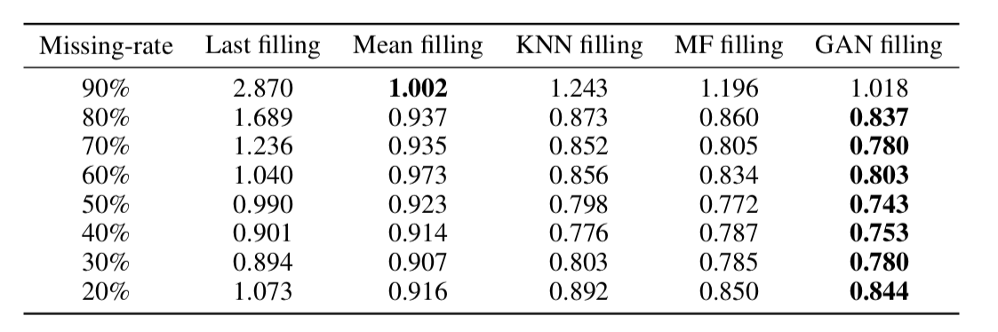
As it turned out, such an approach very adequately recovers data even in time series with a very large proportion of gaps (in the table below - MSE data recovery in the KDD data, depending on the fraction of gaps and recovery method. In most cases, the GAN-based method gives the greatest accuracy recovery).
On the Dimensionality of Word Embeddings
Abstract
Code
Word embedding / vector word representation is an approach widely used for various NLP applications: from recommender systems to analyzing the emotional coloring of texts and machine translation.
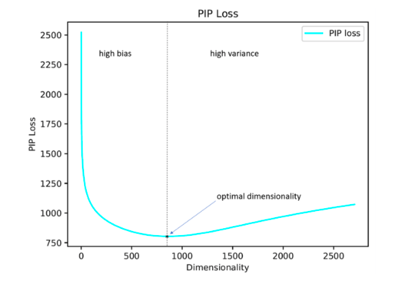
At the same time, the question of how to optimally set such an important hyperparameter as the dimension of vectors remains open. In practice, it is most often selected by empirical brute force or set by default, for example, at the level of 300. At the same time, too small dimension does not reflect all significant interrelationships between words, and too large can lead to retraining.
The authors of the study propose their solution to this problem by minimizing the PIP loss parameter, a new measure of the difference between the two embedding options.
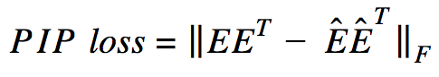
The calculation is based on PIP-matrices, which contain the scalar products of all pairs of vector representations of words in the body. PIP loss is calculated as the Frobenius norm between the PIP-matrices of two embeddings: trained on data (trained embedding E_hat) and perfect, trained on non-noisy data (oracle embedding E).
It would seem that everything is simple: you need to choose a dimension that minimizes PIP loss, the only incomprehensible point is where to get the oracle embedding. In 2015-2017, a number of papers were published in which it was shown that various methods for constructing embeddings (word2vec, GloVe, LSA) implicitly factorize (lower the dimension) the signal matrix of the case. In the case of word2vec (skip-gram), the signal matrix is PMI , in the case of GloVe, the log-counts matrix. It is proposed to take a dictionary of very large size, build a signal matrix and use SVD to obtain oracle embedding. Thus, the dimension of oracle embedding is obtained equal to the rank of the signal matrix (in practice, for a dictionary of 10k words, the dimension will be about 2k). However, our empirical signal matrix is always noisy and we have to resort to clever schemes to get oracle embedding and evaluate the PIP loss using a noisy matrix.
The authors argue that to select the optimal embedding dimension it is enough to use a dictionary of 10k words, which is not very much and allows you to get rid of this procedure in a reasonable time.
As it turned out, the embedding dimension thus calculated in most cases with an error of up to 5% coincides with the optimal dimension, determined on the basis of expert estimates. It turned out (expectedly) that Word2Vec and GloVe practically do not retrain (PIP loss on very large dimensions does not fall), but LSA retrains quite strongly.
With the help of the code laid out by the authors, you can search for the optimal dimension of Word2Vec (skip-gram), GloVe, LSA.
FRAGE: Frequency-Agnostic Word Representation
Abstract
Code
The authors talk about how embeddingings work differently for rare and for popular words. By popular, I mean not stop words (we don’t consider them at all), but meaningful words that are not very rare.
The observations are as follows:
If we talk about popular words, then their proximity is cosine very well reflected.
- their semantic intimacy. For rare words, this is not the case (which is expected), and (which is less expected), the top-n of the closest in cosine measure of words to a rare word is also rare and semantically unrelated. That is, rare and frequent words in the space of embeddingings live in different places (in different cones, if we are talking about cosine)
- During training, vectors of popular words are updated much more often and on average are twice as far from initialization than vectors for rare words. This leads to the fact that the embeddingings of rare words are on average closer to the origin. I, frankly, always thought that, on the contrary, the embeddingings of rare words are, on average, very long , and I don’t know how to treat the authors ’statement =)
Whatever the case with the ratio of embeddingd L2-norms, the separability of popular and rare words is not a very good phenomenon. We want the embeddings to reflect the semantics of the word, not its frequency.
The picture shows popular Word2Vec (red) and rare (blue) words after SVD. Under popular here refers to the top 20% of the words in frequency.
If the problem was only in the L2-norms of embeddings, we could normalize them and live happily, but, as I said in the first paragraph, in cosine proximity (in polar coordinates) rare words are also separated from popular ones.
The authors propose, of course, the GAN. Let's do everything the same as before, but add a discriminator that will try to distinguish popular words from rare ones (again, we consider the top n% words in frequency to be popular).
It looks like this:
The authors test the approach on the tasks of word similarity, machine translation, text classification and language modeling and everywhere perform better baseline. In word similarity it is argued that quality grows especially noticeably in rare words.
One example: citizenship. Skip-gram issues: bliss, pakistans, dismiss, reinforces. FRAGE issues: population, städtischen, dignity, bürger. The words citizen and citizens at FRAGE at 79 and 7 place, respectively (in proximity to the citizenship), at skip-gram - are not in the top 10000.
For some reason, the authors posted the code only for the tasks of machine translation and language modeling, word similarity and text classification in the repository, unfortunately, are not represented.
Unsupervised Cross-Modal Alignment of Speech and Text Embedding Spaces
Abstract
Code: no code, but I would like to
Recent studies have shown that two vector spaces, trained using embedding algorithms (for example, word2vec) on text boxes in two different languages, can be matched to each other without marking and matching the contents of the two bodies to each other. In particular, this approach is used for machine translation in the company Facebook. One of the key properties of embedding spaces is used: inside them, similar words must be geometrically close, and unlike - on the contrary, be far from each other. It is assumed that, in general, the structure of the vector space is preserved regardless of the language in which the corpus was used for learning.
The authors of the article went further and applied a similar approach to the field of automatic speech recognition and translation. It is proposed to teach the vector space separately for the text corpus in the language of interest (for example, Wikipedia), separately for the corpus of recorded speech (in audio format), perhaps in another language, previously broken into words, and then to compare these two spaces similarly to the two text enclosures.
For text body, word2vec is used, and for speech, a similar approach, called Speech2vec, based on LSTM and methodologies used for word2vec (CBOW / skip-gram), so it is assumed that it combines words according to contextual and semantic characteristics, and not sounding.
After both vector spaces are trained and there are two sets of embeddings - S (on the body of speech), consisting of n embeddings of dimension d1 and T (on the body of text), consisting of m embeddings of dimension d2, you need to match them. Ideally, we have a dictionary that determines which vector from S corresponds to which vector from T. Then two matrices are formed for comparison: from S we choose k embeddings that form a matrix X of size d1 xk; from T, too, k embeds are chosen that correspond (in the dictionary) to those previously selected from S, and a matrix Y of size d2 x k is obtained. Next, you need to find a linear mapping W such that:
But since the article discusses the unsupervised approach, there is initially no dictionary, so the procedure for generating a synthetic dictionary, consisting of two parts, is proposed. First, we get the first approximation of W using the domain-adversarial training (competitive model like GAN, only instead of the generator - linear display W, with which we try to make S and T indistinguishable from each other, and the discriminator tries to determine the real origin of embedding). Then, based on the words, the embeddingings of which showed the best fit to each other and are most often found in both cases, a dictionary is formed. After this, W is refined according to the formula above.
This approach gives results comparable to learning on labeled data, which can be very useful in the problem of speech recognition and translation from rare languages for which there are too few parallel speech-text shells, or they are missing.
Deep Anomaly Detection Using Geometric Transformations
Abstract
Code
An unusual approach to anomaly detection, which, according to the authors, greatly overcomes other approaches.
The idea is this: let's invent K different geometric transformations (combinations of shifts, rotate 90 degrees and reflections) and apply them to each picture of the original dataset. The picture resulting from the i-th transformation will now belong to class i, that is, there will be K classes in total, each of them will be represented by such a number of pictures that was originally in dataset. Now we will teach a multi-class classification on such markup (the authors chose wide resnet).
Now we can get K vectors y (Ti (x)) of dimension K, where Ti is the i-th transformation, x is the picture, y is the output of the model. The basic definition of “normality” is as follows:
Here, for the image x, we add the predicted probabilities of the correct classes for all transformations. The greater the “normality”, the more likely it is that the image is taken from the same distribution as the training sample. The authors claim that it already works very well, but nevertheless they offer a more complex way that works even better. We will assume that the vector y (Ti (x)) for each transformation Ti is distributed over Dirichlet and as a measure of the “normality” of the image we will consider the log likelihood. The Dirichlet distribution parameters are estimated on the training set.
The authors report an incredible boost of performance compared to other approaches.
A Simple Unified Framework for Detecting Out of Distribution and Adversarial Attacks
Abstract
Code
Identifying cases in a sample for applying a model that is significantly different from the distribution of a training sample is one of the basic requirements for obtaining reliable classification results. At the same time, neural networks are known for their feature with a high degree of certainty (and incorrectly) to classify objects that have not been encountered in training, or that are intentionally destructive (adversarial examples).
The authors of the article propose a new method of identifying both those and other "bad" cases. The approach is implemented as follows: first, the neural network is trained with the usual softmax output, then the output of its penultimate layer is taken, and the generative classifier is trained on it. Let there be x - what is fed to the input of the model for a specific classification object, y is the corresponding class label, then suppose that we have a pre-trained softmax classifier of the form:
Where wc and bc are weights and softmax layer constant for class c, and f (.) Is the output of the last but one soybean DNN.
Further, without any changes to the pre-trained classifier, a transition is made to the generative classifier, namely discriminant analysis. It is assumed that the signs taken from the penultimate layer of the softmax classifier have a multidimensional normal distribution, each component of which corresponds to one class. Then the conditional distribution can be defined through the vector of averages of the multidimensional distribution and its covariance matrix:
To estimate the parameters of the generative classifier, empirical averages are calculated for each class, as well as the covariance for cases from the training set {(x1, y1), ..., (xN, yN)}:
where N is the number of cases of the corresponding class in the training sample. Then, on the test sample, a measure of reliability is calculated - the Mahalanobis distance between the test case and the normal distribution of the class closest to this case.
As it turned out, such a metric works much more reliably on atypical or spoiled objects, without giving overestimated estimates, as in the softmax layer. In most comparisons on different data, the proposed method showed results that exceeded the current state-of-the-art in finding both cases that were not in training, and intentionally spoiled.
Next, the authors consider another interesting application of their methodology: use the generative classifier to highlight new classes on the test, which were not in training, and then update the parameters of the classifier itself so that it can later determine this new class.
Adversarial Examples that Fool both Computer Vision and Time-Limited Humans
Abstract: https://arxiv.org/abs/1802.08195
The authors investigate what adversarial examples are from the point of view of human perception. Today, no one is surprised by the fact that it is possible almost without changing the image to make the network make mistakes on it. However, it is not very clear how the original picture differs from the adversarial example for a person and if it differs at all. It is clear that none of the people will call the picture on the right an ostrich, but still, perhaps the picture on the right for a person is not exactly identical to the picture on the left, and, if so, a person can also be exposed to adversarial attacks.
The authors try to assess how well a person can classify adversarial examples. To obtain adversarial examples, a technique is used which does not have access to the architecture of the original network (the authors' logic is that they still will not be given access to the architecture of the human brain).
So, a person is shown adversarial example, as in the picture above and asked to classify it. It is clear that in normal conditions the result would be predictable, but here one image is shown to a person for 63 milliseconds after which he must choose one of two classes. In such conditions, the accuracy of the original images was 10% higher than the adversarial. In principle, this could be explained by the fact that the adversarial image is simply noisy and therefore, in the conditions of a shortage of time, people incorrectly classify it, but this refutes the following experiment. If, before adding perturbation to the image, we reflect this perturbation vertically, then accuracy will hardly change compared to the original image.
On the histogram adv - adversarial example, image - the original image, flip - the original image + adversarial perturbation, reflected vertically.
Sanity Checks for Saliency Maps
Abstract
Interpretation of models is one of the most discussed topics today. If we are talking about deep learning, we usually talk about saliency maps. Saliency maps try to answer the question of how the value changes at one of the grid outputs when the input values change. This may look like a saliency map, which shows which pixels affected the image being classified as a “dog”.
The authors ask a very reasonable question: “How would we validate the methods of constructing saliency maps?” Two obvious theses are put forward that are proposed to be tested:
- Saliency map must depend on grid weights.
- Saliency map should depend on the laws that are in the data
We will check the first thesis, replacing the weights in the trained grid with randomization: cascading randomization (random layers, starting with the last one and see how the saliency map changes) and independent randomization (random random layers). The second thesis will be checked like this: randomly we mix all the labels on the train, overfit the train and look at the saliency maps.
If the method of constructing a saliency map is really good and allows you to understand how the model works, such randomization should greatly change the saliency maps. However: “To our surprise, some widely deployed,” the authors state. Here, for example, how saliency maps, obtained using various algorithms, after cascading randomization look like:
Note the funny fact that the last column corresponds to a grid with random weights in all layers. That is, the grid predicts randomly, but some saliency maps still draw a bird.
The authors rightly say that - assessment of saliency maps by their comprehensibility and consistency and insufficient attention to the extent to which the result is related to how the model works leads to a confirmation bias. Apparently, including for this reason, it turns out that common approaches to the interpretation of models do not interpret them at all.
An intriguing failing of convolutional neural networks and the CoordConv solution
Abstract: https://arxiv.org/abs/1807.03247
Code: there are already many implementations, and in general the idea is so beautiful and simple that it is written literally in 10 lines.
A simple and promising idea from Uber. Convolutional networks are initially sharpened for shear invariance, so the tasks associated with determining the coordinates of an object for such networks are very difficult. Ordinary convolutional networks are not able to solve even toy problems such as determining the coordinates of a point in a picture or drawing a point along coordinates:
A very elegant hack is proposed: add to the picture (in general, to the CoodrConv layer input) two matrices i and j, which will contain the vertical and horizontal coordinates of the corresponding pixels:
It is alleged that:
- Such convolutions do not spoil the performance on ImageNet. The task of classifying images just requires shift invariance, and, judging by the results, the grid easily learns that you don’t need to use coordinates in the classification task
- CoordConv greatly improves object detection. According to the results of experiments on the detection of numbers from MNIST, scattered throughout the picture with the help of Faster R-CNN, declare an increase in IoU by 21%
- When using CoordConv in GAN, the variety of generated images increases.
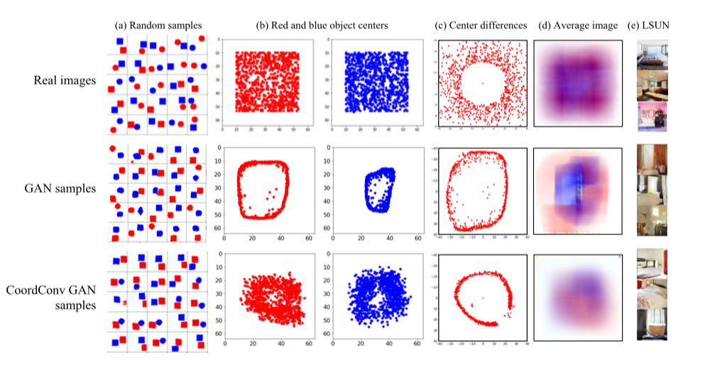
We trained GANs in two datasets: a toy dataset with red and blue figures in random places and a dataset with LSUN bedroom interiors. In the first dataset, the centers of the figures are evenly distributed, the distribution of the difference between the centers is the upper graph in column c. Given that the samples generated by GAN'om are similar to the original ones, it can be seen that the distribution of centers and distances between the centers is very different. When using CoordConv, the distribution of distances between centers is much more similar to the original, although problems with distance differences remain. In the case of LSUN on column d, it can be seen that, in general, the distribution of samples generated by the CoordConv GAN is closer to the original - 4. Using CoordConv in A2C gives a boost in some (not all) games.
Personally, the second point is more interesting to me from this, I would like to see the results on real datasets, but at the same time nothing is googled. Meanwhile, CoordConv is already actively building in U-net : https://arxiv.org/abs/1812.01429, https://www.kaggle.com/c/tgs-salt-identification-challenge/discussion/69274 , https: //github.com/mjDelta/Kaggle-RSNA-Pneumonia-Detection-Challenge .
There is a good and more detailed video from the author .
Regularizing by the Variance of the Activations' Sample-Variances
Abstract
Code
The authors offer a fun alternative to batch normalization. We will fine the grid for the variability of the dispersion of activations on some layer. : S1 S2 :
σ2 — S1 S2 , β — . variance constancy loss (VCL) .
, (). 11- (CIFAR-10 CIFAR-100). , VCL , Leaky ReLU ELU, ReLU batch normalization. 2 Tiny Imagenet — Imagenet 200 64x64. VCL batch normalization ELU, ResNet-110 DenseNet-40, Wide-ResNet-32. , , S1 S2 .
VCL feed-forward VCL , batch normalization .
DropMax: Adaptive Variational Softmax
Abstract
- . , , . , “” , .
MNIST, CIFAR Imagenet , DropMax SoftMax, .
Accurate Intelligible Models with Pairwise Interactions
(Friends Don't Let Friends Deploy Black-Box Models: The Importance of Intelligibility in Machine Learning)
Abstract: http://www.cs.cornell.edu/~yinlou/papers/lou-kdd13.pdf
: . , . , =)
, : https://github.com/dswah/pyGAM . feature interactions ( GAM GA2M).
“Interpretability and Robustness in Audio, Speech, and Language”, , ., - . , , . « », , , , , , . , , , - , . .
, : . : , , . , , , . xgboost , , , , , .
, , — GA2M, (Generalized additive models).
GAM , GLM: , , , GLM, ( , – , «»). GAM , . , () .
GAM « ». , – , , – , . GA2M.
GAM ( ), ( GAM). , , FAST, .
, . , GA2M c FAST .
, . , , 20 ( UCI). : 2018 . 50 — , .
— . . , , , , — black-box . , , , .
, . . 10 ( L2- ), , , predict_proba 0.86. , sparse . , L1-, . L1- . 0, , , . , . , interpretable and credible models .
Visualization for Machine Learning: UMAP
Absract
“Visualization for Machine Learning” Google Brain. , , , , , – , , , .., . , .
, Uniform Manifold Approximation and Projection (UMAP) – . , , , . , UMAP t-SNE 2-10 , , :
, t-SNE UMAP , (. . ), ( ) — , .
, UMAP , t-SNE: , MNIST Fashion MNIST UMAP:
— : UMAP sklearn, sklearn pipeline. , , UMAP , t-SNE, .. .
semi-supervised — , UMAP .
? , , .
Source: https://habr.com/ru/post/434694/
All Articles