Introduction to Performance Research

When developing a product, they rarely pay due attention to its performance at high intensity of incoming requests. This is done very little or not at all - there is not enough time, or specialists are justified by the typical phrase: “We work fast and everything works fast, why check something else?”. In such cases, there may come a time when a well-functioning production suddenly falls due to the surging flow of visitors, for example, under the Habraeffect. Then it becomes clear that doing performance research is really necessary.

This task confuses many people, because there is a need, but there is no clear understanding of what should be measured and how to interpret the result, sometimes there are not even formed non-functional requirements. Next, I will talk about how to start if you decide to go this way, and explain which metrics are important in researching performance, and how to use them.

Some theory

Imagine that we have a spherical application in a vacuum — it receives requests and gives answers to them. For simplicity, it can be a microservice with one method that does not go anywhere and does not depend on other components or applications. In this case, we are not interested in what it is written on, how it works, and in what environment it is launched.

What do we want to know about performance? It is probably good to know the maximum flow of incoming requests, at which the service is stable, its performance in this thread and the time it takes to execute a single request. It’s very good if you can identify the reasons that limit further productivity growth.

Obviously, it is necessary to measure the response time to a request, respectively, the flow of incoming requests or intensity will be understood as the number of requests per unit of time, as a rule, per second, and by performance, the number of responses in the same time unit. Response times can be scattered over a wide range, so for a start it makes sense to present them as an average per second.

In addition, problems can arise at various levels: starting with the fact that the service responds with an error (and it’s good if it’s five hundred, rather than “200 OK {" status ":" error "}"), and ending with stops responding altogether or answers start getting lost at the network level. Unsuccessful requests need to be able to catch, and it is convenient to represent them as a percentage of the total. A graph of performance, response time and error rate versus intensity looks like this:

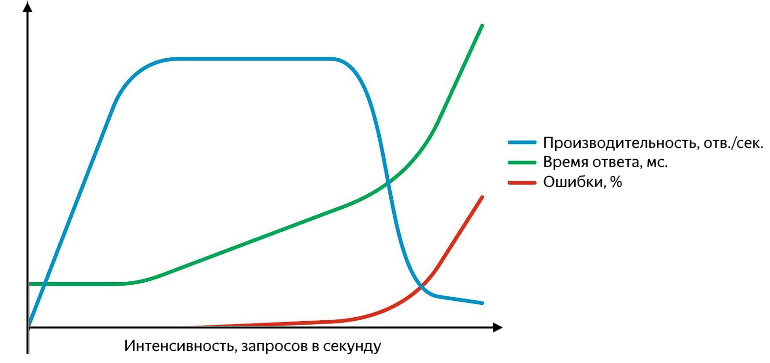
As the intensity of requests grows, response times and error rates increase.

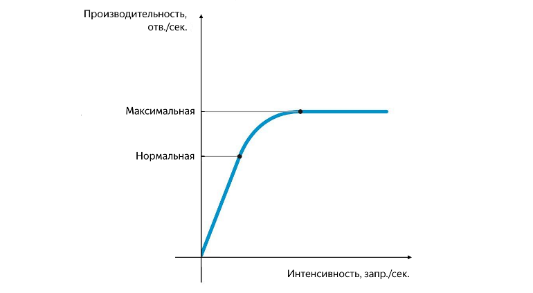
While productivity is growing in a linear dependence on intensity - the service is all right. It successfully processes the entire incoming flow of requests, the response time does not change, there are no errors. Continuing to increase the intensity, we obtain a slowdown in productivity growth until the moment of saturation, in which productivity reaches its maximum and the response time begins to increase. A subsequent increase in intensity will lead to a breakdown - a significant increase in response time and a drop in performance, and an active increase in errors will begin. At the stage of growth and saturation, there are two important points - normal and maximum performance.

Normal and maximum performance

Normal productivity is reached at the moment when the rate of its growth begins to decrease, and maximum - at the moment when the rate of its growth vanishes. The division of performance into normal and maximum is very important. At an intensity that corresponds to normal performance, the application should work stably, and the value of normal performance characterizes the threshold after which the bottleneck of the service begins to appear, having a negative impact on its operation. When the maximum performance is reached, the bottleneck begins to completely restrict further growth, the work of the service is unstable, and, as a rule, at this moment even a small but stable background of errors begins to appear.

The problem can be caused by various reasons - queues are clogged, there are not enough threads, the pool is exhausted, the CPU or RAM is fully utilized, insufficient read / write speed from the disk and the like. It is important to understand that the correction of one bottleneck will lead to the fact that the performance will be limited by the next and so on. Completely get rid of the bottleneck can not, it can only be transferred.

Experiments

First of all, it is necessary to determine the intensity at which the service reaches normal and maximum performance, and the corresponding average response time. To do this, in the experiment it is enough to simply increase the flow of incoming requests. It is more difficult to determine the value of the maximum intensity and the time of the experiment.

You can build on what is written in the non-functional requirements (if any), on the maximum user load from the sale, or simply take values ​​from the ceiling. If the intensity of the incoming flow is not enough - the service does not have time to reach saturation and it will be necessary to repeat the experiment. If the intensity is too high, the service will very quickly reach saturation, and then degradation. In such a case, it is convenient to have monitoring so that, with a significant increase in the number of errors, do not waste time in vain and stop the experiment.

In our experiments, we smoothly increase the intensity from 0 to 1000 requests per second for 10 minutes. This is enough for the service to reach saturation, and then, if necessary, adjust the time and intensity value in the next experiment to get a more accurate result. On the graphs above everything was smooth and beautiful, but in the real world it is difficult at first glance to determine the value of normal performance.

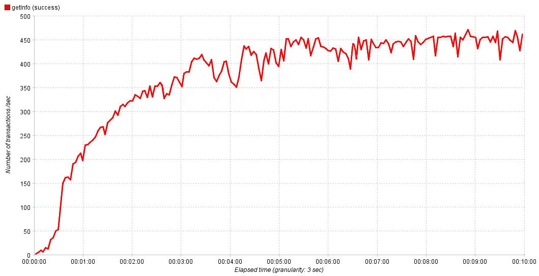
Real service performance versus time

We then take 80-90% of the maximum for normal performance. If, after reaching saturation, we observe active growth of errors, it makes sense to investigate them, because they are a consequence of a bottleneck, their study will help to localize it and transfer it to correction.

So, the first results are obtained. We now know the normal and maximum performance of the application, as well as the response times corresponding to them. That's all? Of course not! With normal performance, the service should work stably, which means that it is necessary to check its operation under normal load for some time. Which one You can again look in the non-functional requirements, ask analysts or monitor the duration of the periods of maximum activity on the prod. In our experiments, we linearly increase the load from 0 to normal and withstand it for 10-15 minutes. This is sufficient if the maximum user load is substantially less than normal, but if they are comparable, the experiment time should be increased.

To quickly evaluate the result of the experiment, it is convenient to aggregate the data obtained in the form of the following metrics:

• average response time
• median,
• 90% percentile,
• % of errors
• performance.

What is the average response time is understandable; however, the average is an adequate measure only in the case of a normal distribution of the sample, since it is too sensitive to “outliers” - too large or too small values ​​that are strongly out of the general trend. The median is the middle of the entire sample of response times, half the values ​​are less than it, the rest is more. Why is it needed?

Firstly, based on its definition, it is less sensitive to emissions, that is, it is a more adequate metric, and secondly, by comparing it with the average, you can quickly evaluate the response distribution characteristic. In an ideal situation, they are equal - the distribution of response times is normal, and the service is fine!

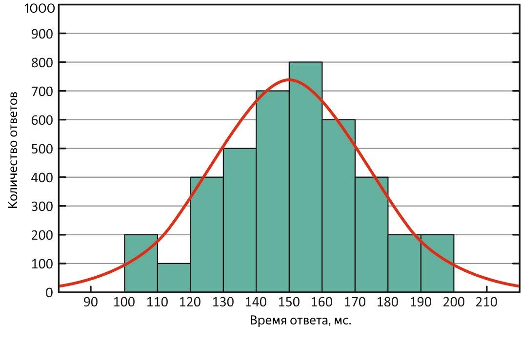
Normal distribution of response times. With this distribution, the mean and median are equivalent

If the mean is very different from the median, then the distribution is skewed, and in the course of the experiment there could be “outliers”. If the average is greater - there were periods when the service responded very slowly, in other words, it slowed down.

Distribution of response times with “outliers” of long responses. With this distribution, the average is greater than the median.

Such cases require additional analysis. To estimate the scale of “emissions”, quantiles or percentiles come to the rescue.

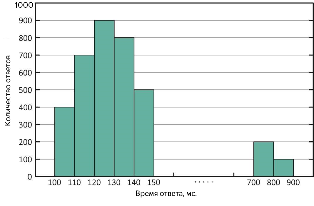
The quantile, in the context of the received sample, is the value of the response time to which the corresponding part of all requests fits. If% of queries is used, then this is percentile (by the way, the median is 50% percentile). To estimate the "emissions" is convenient to use the 90% percentile. For example, as a result of the experiment, a median of 100 ms was obtained, and the average was 250 ms, 2.5 times the median! Obviously, this is not very good, we look at 90% quantile, and there 1000 ms - as many as 10% of all successful queries ran for more than a second, disarray, we need to understand. To search for long requests, you can click on the file with the results of the experiment or immediately on the service logs, but it is even better to present the average response time as a graph of time dependence, it will immediately show both the time and the nature of the “outliers”.

Results

So, you have successfully conducted experiments and obtained results. A good result or a bad one depends on the requirements that are imposed on the service, but it’s much more important not to get the numbers, but why these numbers are, and how the further growth is limited. If you managed to find a bottleneck - very good, if not, then sooner or later the need for performance may increase, and you will still have to look for it, so sometimes it is easier to prevent the situation.

In this article, I gave a basic approach to performance research, answering questions that I had at the very beginning. Do not be afraid to explore the performance, it is necessary!

PS
Come to our cozy telegram chat , where you can ask questions, help with advice and just talk about performance research.