Is it possible to train with reinforcements agent for trading in the stock market? R language implementation
Let's create a prototype of a learning agent with reinforcements (RL) who will master the skill of trading.
Given that the implementation of the prototype works in the R language, I urge R users and programmers to come closer to the ideas presented in this material.
This is a translation of my English-language article: Can Reinforcement Learning Trade Stock? Implementation in R.
')
I want to warn code hunters that in this note there is only a neural network code adapted for R.
If I did not distinguish myself in good Russian, point out the mistakes (the text was prepared with the help of an automatic translator).
I advise you to start the dive into the topic with this article: DeepMind
It will introduce you to the idea of using the Deep Q-Network (DQN) to approximate the value function, which are crucial in Markov decision-making processes.
I also recommend delving into math using the preprint of this book by Richard S. Sutton and Andrew J. Barto: Reinforcement Learning
Below I will present an extended version of the original DQN, which includes more ideas that help the algorithm to quickly and efficiently converge, namely:
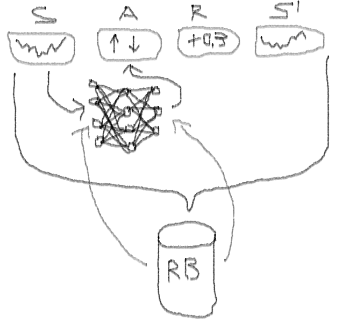
Deep Double Dueling Noisy NN neural networks with a priority selection from the experience playback buffer.
What makes this approach better than classic DQN?
There are reasons why this is interesting:
In order not to stretch the material, look at the code of this NN, which I want to share, since this is one of the mysterious parts of the whole project.
I used this source to adapt the Python code for the noise part of the network: github repo
This neural network looks like this:
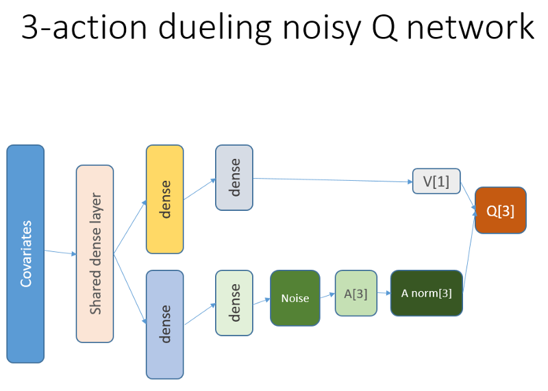
Recall that in the duel architecture, we use equality (equation 1):
Q = A '+ V, where
A '= A - avg (A);
Q = state-action value;
V = state value;
A = advantage.
Other variables in the code speak for themselves. In addition, this architecture is only good for a specific task, so do not take it for granted.
The rest of the code is likely to be quite template for publication, and it will be interesting for the programmer to write it yourself.
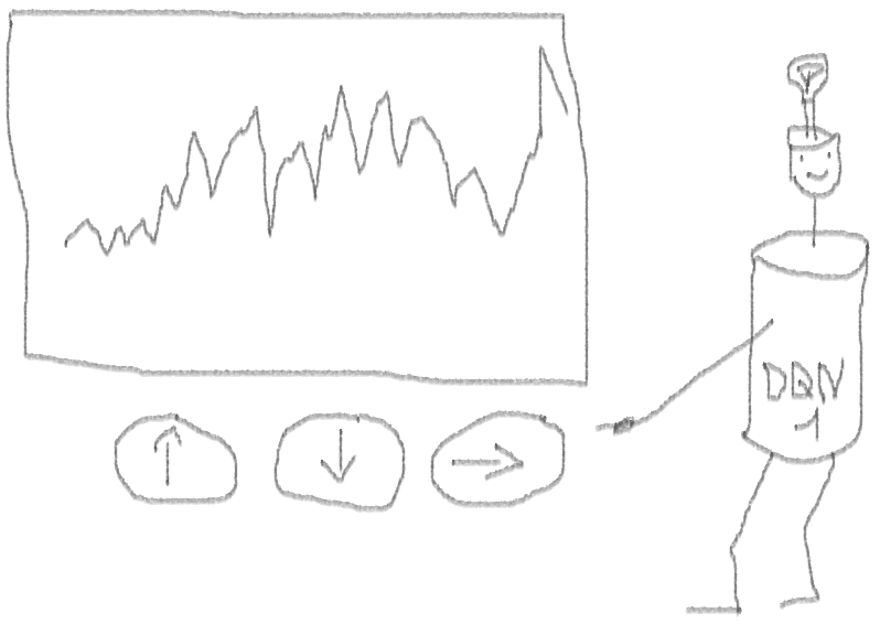
And now - experiments. Testing the work of the agent was carried out in a sandbox, far from the realities of trading in a live market, with a real broker.
We run our agent vs synthetic dataset. Our transaction value is 0.5:
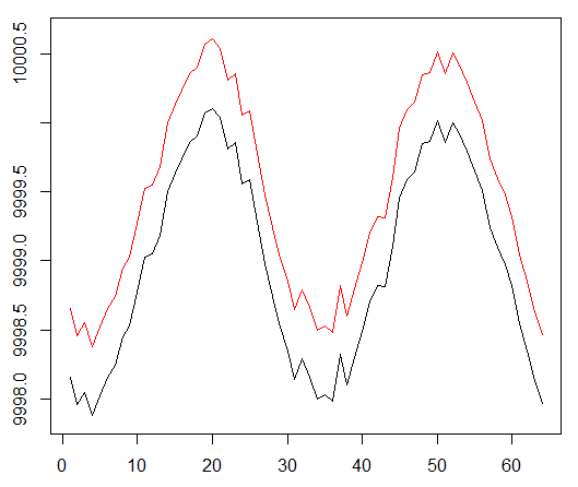
The result is excellent. The maximum average episodic reward in this experiment
should be 1.5.
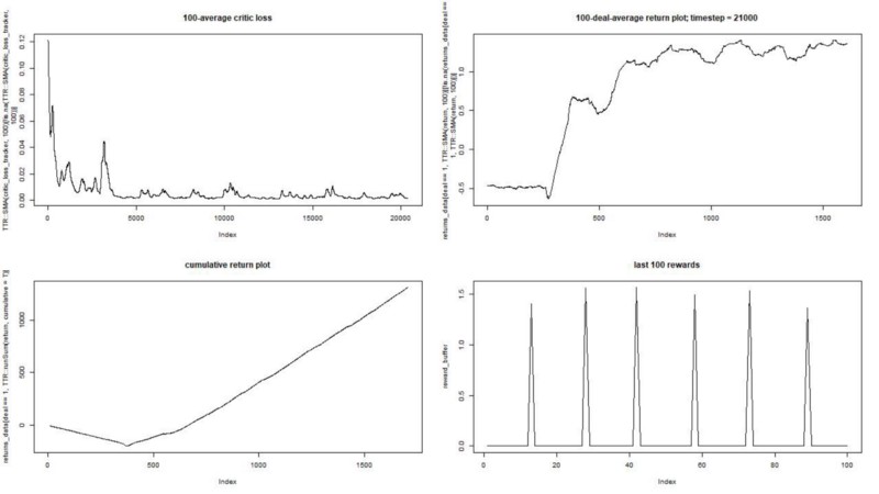
We see: the loss of the critic (the so-called network of values in the approach of the actor-critic), the average remuneration for the episode, the cumulative reward, the sample of the last rewards.
We train our agent to an arbitrarily chosen exchange symbol, which demonstrates interesting behavior: a smooth start, fast growth in the middle and a dreary end. In our training set about 4300 days. Transaction cost is set at 0.1 USD (purposefully low); the reward is USD Profit / loss after closing a deal to buy / sell 1.0 shares.
Source: finance.yahoo.com/quote/algn?ltr=1
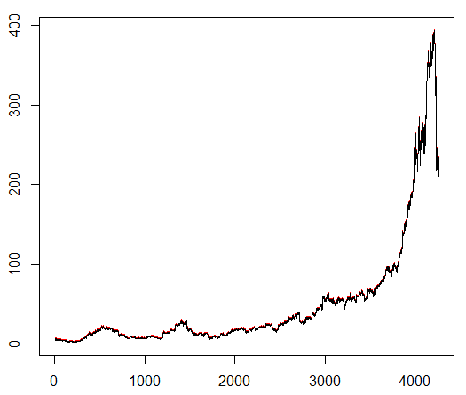
NASDAQ: ALGN
After configuring some parameters (leaving the NN architecture the same), we arrived at the following result:

It turned out not bad, because in the end the agent learned to make a profit by pressing the three buttons on his console.
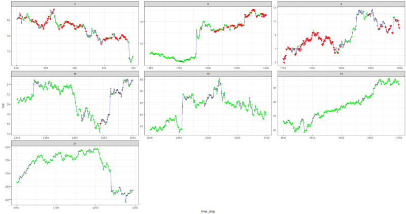
red marker = sell, green marker = buy, gray marker = do nothing.
Note that at its peak, the average reward for an episode exceeded the realistic value of the transaction, which can be encountered in real trading.
It is a pity that stocks are falling like crazy because of bad news ...
Trading with RL is not only difficult, but also useful. When your robot does it better than you, it's time to spend personal time to get an education and health.
I hope it was an interesting journey for you. If you like this story, wave your hand. If there is a lot of interest, I can continue and show you how policy gradient methods work using the R language and the Keras API.
I also want to thank my friends who are passionate about neural networks for their advice.
If you have any questions, I am always here.
Given that the implementation of the prototype works in the R language, I urge R users and programmers to come closer to the ideas presented in this material.
This is a translation of my English-language article: Can Reinforcement Learning Trade Stock? Implementation in R.
')
I want to warn code hunters that in this note there is only a neural network code adapted for R.
If I did not distinguish myself in good Russian, point out the mistakes (the text was prepared with the help of an automatic translator).
Introduction to the problem
I advise you to start the dive into the topic with this article: DeepMind
It will introduce you to the idea of using the Deep Q-Network (DQN) to approximate the value function, which are crucial in Markov decision-making processes.
I also recommend delving into math using the preprint of this book by Richard S. Sutton and Andrew J. Barto: Reinforcement Learning
Below I will present an extended version of the original DQN, which includes more ideas that help the algorithm to quickly and efficiently converge, namely:
Deep Double Dueling Noisy NN neural networks with a priority selection from the experience playback buffer.
What makes this approach better than classic DQN?
- Dual: there are two networks, one of which is trained, and the other estimates the following values of Q
- Dueling: there are neurons that clearly appreciate the value and benefits
- Noisy: there are noise matrices applied to the weights of the intermediate layers, where the mean and standard deviations are learning weights
- Sampling priority: batches of observations from the playback buffer contain examples, due to which previous training of functions led to large residues that can be stored in an auxiliary array.
Well, what about the trade done by the DQN agent? This is an interesting topic as such.
There are reasons why this is interesting:
- Absolute freedom of choice of representations of the state, actions, awards and architecture NN. You can enrich the entry space with anything you consider worth trying, from news to other stocks and indices.
- Compliance of the trading logic with the reinforcement learning logic is that: the agent performs discrete (or continuous) actions, is rarely rewarded (after closing the transaction or expiration of the period), the environment is partially observable and may contain information on the next steps, trading is an episodic game.
- You can compare the results of DQN with several references, such as indices and technical trading systems.
- The agent can continuously learn new information and, thus, adapt to the changing rules of the game.
In order not to stretch the material, look at the code of this NN, which I want to share, since this is one of the mysterious parts of the whole project.
R-code for value neural network using Keras to build our agent RL
Code
# configure critic NN ------------ library('keras') library('R6') learning_rate <- 1e-3 state_names_length <- 12 # just for example a_CustomLayer <- R6::R6Class( "CustomLayer" , inherit = KerasLayer , public = list( call = function(x, mask = NULL) { x - k_mean(x, axis = 2, keepdims = T) } ) ) a_normalize_layer <- function(object) { create_layer(a_CustomLayer, object, list(name = 'a_normalize_layer')) } v_CustomLayer <- R6::R6Class( "CustomLayer" , inherit = KerasLayer , public = list( call = function(x, mask = NULL) { k_concatenate(list(x, x, x), axis = 2) } , compute_output_shape = function(input_shape) { output_shape = input_shape output_shape[[2]] <- input_shape[[2]] * 3L output_shape } ) ) v_normalize_layer <- function(object) { create_layer(v_CustomLayer, object, list(name = 'v_normalize_layer')) } noise_CustomLayer <- R6::R6Class( "CustomLayer" , inherit = KerasLayer , lock_objects = FALSE , public = list( initialize = function(output_dim) { self$output_dim <- output_dim } , build = function(input_shape) { self$input_dim <- input_shape[[2]] sqr_inputs <- self$input_dim ** (1/2) self$sigma_initializer <- initializer_constant(.5 / sqr_inputs) self$mu_initializer <- initializer_random_uniform(minval = (-1 / sqr_inputs), maxval = (1 / sqr_inputs)) self$mu_weight <- self$add_weight( name = 'mu_weight', shape = list(self$input_dim, self$output_dim), initializer = self$mu_initializer, trainable = TRUE ) self$sigma_weight <- self$add_weight( name = 'sigma_weight', shape = list(self$input_dim, self$output_dim), initializer = self$sigma_initializer, trainable = TRUE ) self$mu_bias <- self$add_weight( name = 'mu_bias', shape = list(self$output_dim), initializer = self$mu_initializer, trainable = TRUE ) self$sigma_bias <- self$add_weight( name = 'sigma_bias', shape = list(self$output_dim), initializer = self$sigma_initializer, trainable = TRUE ) } , call = function(x, mask = NULL) { #sample from noise distribution e_i = k_random_normal(shape = list(self$input_dim, self$output_dim)) e_j = k_random_normal(shape = list(self$output_dim)) #We use the factorized Gaussian noise variant from Section 3 of Fortunato et al. eW = k_sign(e_i) * (k_sqrt(k_abs(e_i))) * k_sign(e_j) * (k_sqrt(k_abs(e_j))) eB = k_sign(e_j) * (k_abs(e_j) ** (1/2)) #See section 3 of Fortunato et al. noise_injected_weights = k_dot(x, self$mu_weight + (self$sigma_weight * eW)) noise_injected_bias = self$mu_bias + (self$sigma_bias * eB) output = k_bias_add(noise_injected_weights, noise_injected_bias) output } , compute_output_shape = function(input_shape) { output_shape <- input_shape output_shape[[2]] <- self$output_dim output_shape } ) ) noise_add_layer <- function(object, output_dim) { create_layer( noise_CustomLayer , object , list( name = 'noise_add_layer' , output_dim = as.integer(output_dim) , trainable = T ) ) } critic_input <- layer_input( shape = c(as.integer(state_names_length)) , name = 'critic_input' ) common_layer_dense_1 <- layer_dense( units = 20 , activation = "tanh" ) critic_layer_dense_v_1 <- layer_dense( units = 10 , activation = "tanh" ) critic_layer_dense_v_2 <- layer_dense( units = 5 , activation = "tanh" ) critic_layer_dense_v_3 <- layer_dense( units = 1 , name = 'critic_layer_dense_v_3' ) critic_layer_dense_a_1 <- layer_dense( units = 10 , activation = "tanh" ) # critic_layer_dense_a_2 <- layer_dense( # units = 5 # , activation = "tanh" # ) critic_layer_dense_a_3 <- layer_dense( units = length(acts) , name = 'critic_layer_dense_a_3' ) critic_model_v <- critic_input %>% common_layer_dense_1 %>% critic_layer_dense_v_1 %>% critic_layer_dense_v_2 %>% critic_layer_dense_v_3 %>% v_normalize_layer critic_model_a <- critic_input %>% common_layer_dense_1 %>% critic_layer_dense_a_1 %>% #critic_layer_dense_a_2 %>% noise_add_layer(output_dim = 5) %>% critic_layer_dense_a_3 %>% a_normalize_layer critic_output <- layer_add( list( critic_model_v , critic_model_a ) , name = 'critic_output' ) critic_model_1 <- keras_model( inputs = critic_input , outputs = critic_output ) critic_optimizer = optimizer_adam(lr = learning_rate) keras::compile( critic_model_1 , optimizer = critic_optimizer , loss = 'mse' , metrics = 'mse' ) train.x <- rnorm(state_names_length * 10) train.x <- array(train.x, dim = c(10, state_names_length)) predict(critic_model_1, train.x) layer_name <- 'noise_add_layer' intermediate_layer_model <- keras_model(inputs = critic_model_1$input, outputs = get_layer(critic_model_1, layer_name)$output) predict(intermediate_layer_model, train.x)[1,] critic_model_2 <- critic_model_1 I used this source to adapt the Python code for the noise part of the network: github repo
This neural network looks like this:
Recall that in the duel architecture, we use equality (equation 1):
Q = A '+ V, where
A '= A - avg (A);
Q = state-action value;
V = state value;
A = advantage.
Other variables in the code speak for themselves. In addition, this architecture is only good for a specific task, so do not take it for granted.
The rest of the code is likely to be quite template for publication, and it will be interesting for the programmer to write it yourself.
And now - experiments. Testing the work of the agent was carried out in a sandbox, far from the realities of trading in a live market, with a real broker.
Phase I
We run our agent vs synthetic dataset. Our transaction value is 0.5:
The result is excellent. The maximum average episodic reward in this experiment
should be 1.5.
We see: the loss of the critic (the so-called network of values in the approach of the actor-critic), the average remuneration for the episode, the cumulative reward, the sample of the last rewards.
Phase II
We train our agent to an arbitrarily chosen exchange symbol, which demonstrates interesting behavior: a smooth start, fast growth in the middle and a dreary end. In our training set about 4300 days. Transaction cost is set at 0.1 USD (purposefully low); the reward is USD Profit / loss after closing a deal to buy / sell 1.0 shares.
Source: finance.yahoo.com/quote/algn?ltr=1
NASDAQ: ALGN
After configuring some parameters (leaving the NN architecture the same), we arrived at the following result:
It turned out not bad, because in the end the agent learned to make a profit by pressing the three buttons on his console.
red marker = sell, green marker = buy, gray marker = do nothing.
Note that at its peak, the average reward for an episode exceeded the realistic value of the transaction, which can be encountered in real trading.
It is a pity that stocks are falling like crazy because of bad news ...
Concluding remarks
Trading with RL is not only difficult, but also useful. When your robot does it better than you, it's time to spend personal time to get an education and health.
I hope it was an interesting journey for you. If you like this story, wave your hand. If there is a lot of interest, I can continue and show you how policy gradient methods work using the R language and the Keras API.
I also want to thank my friends who are passionate about neural networks for their advice.
If you have any questions, I am always here.
Source: https://habr.com/ru/post/433182/
All Articles