Open lesson "Feature Engineering on the example of the classic dataset of the Titanic"
Hello again!
In December, we will start training the next Data Scientist group , so there are more and more open lessons and other activities. For example, just recently, a webinar was held under the long title “Feature Engineering on the example of the classic Titanic dataset”. It was conducted by Alexander Sizov - an experienced developer, Ph.D., an expert on Machine / Deep learning and a participant in various commercial international projects related to artificial intelligence and data analysis.
Open lesson took about one and a half hours. During the webinar, the teacher spoke about the selection of signs, the transformation of the source data (coding, scaling), setting parameters, training the model and much more. In the course of the lesson, the participants were shown a Jupyter Notebook. Open source data from the Kaggle platform (a classic dataset about “Titanic”, from which many begin their acquaintance with Data Science) was used for work. Below we offer a video and transcript of the past event, and here you can pick up the presentation and codes in the Jupiter's laptop.
')
Feature selection
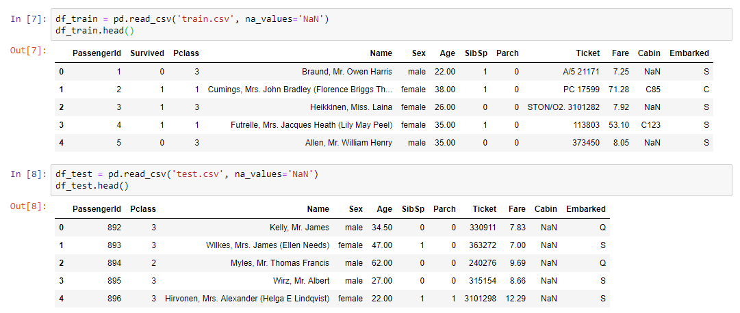
The topic was chosen, although classical, but still a bit gloomy. In particular, it was necessary to solve the problem of binary classification and predict according to the available data whether a passenger will survive or not. The data itself was divided into two samples, Training and Test. The key variable is Survival (survived / not survived; 0 = No, 1 = Yes).
Input training data:
As you can see, the types of variables are different: numeric, text. From this kaleidoscope it was necessary to form a dataset for the upcoming training of the model.
We summarize:
Work algorithm
The practical part of the webinar
The first thing that needed to be done was to read the dataset and display our data on the screen:
For data analysis, a little-known but quite useful profiling library was used:
Read more about profiling
This library does everything that can be done a priori without knowing the details about the data. For example, display statistics on data (how many variables and what type they are, how many lines, missing values, etc.). Moreover, separate statistics are given for each variable with the reduction of the minimum and maximum, the distribution graph, and other parameters.
As you know, in order to make a good model, you need to understand the process that we are trying to model and understand which features are key. And by no means always in our data there is everything that is needed, or, more precisely, almost never they lack all the necessary, fully determining and determining our process. As a rule, we always need to combine something, perhaps, to add additional features that are not represented in the dataset (say, the weather forecast). It is to understand the process and need data analysis, which can be done using the profiling library.
Missing values
The next step is to solve the problem of missing values, because in most cases the data is not completely filled.
There are the following solutions to this problem:
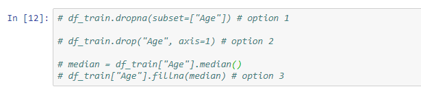
An example of a simple conversion using the fillna method, which assigns the values of the median variable to only those cells that are not filled:
In addition, the teacher showed examples of using Imputer and pipeline.
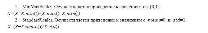
Feature scaling
The work of the model and the final decision depends on the scale of the signs. The fact is that it is not a fact that any sign, which has a larger scale, is more important than a sign, which has a smaller scale. That is why models need to submit attributes that are scaled in the same way, that is, having the same weight for the model.
There are different scaling techniques, but the format of the open lesson allowed us to consider in more detail only two of them:
Combinations of signs
Combinations of existing features using arithmetic operations (sum, multiplication, division) allow to obtain any feature that makes the model more efficient. This is not always possible, and we do not know which combination will give the desired effect, but practice shows that it makes sense to try. It is convenient to apply transformations of signs using the pipeline.
Coding
So, we have data of different types: numeric and text. Currently, most models on the market cannot work with textual data. As a result, all categorical features (textual) must be converted to a numerical representation, for which encoding is used.
Label encoding . This is the mechanism implemented in many libraries, which can be called and applied:
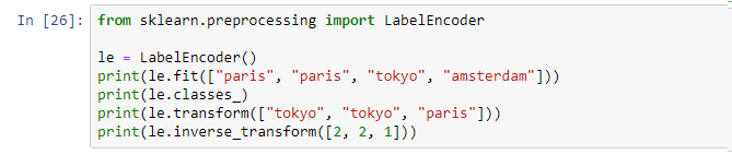
Label encoding assigns a unique identifier to each unique value. Minus - we bring order into some variable that was not ordered, which is not good.
OneHotEncoder. Unique text variable values are expanded as columns, which are added to the source data, where each column is a binary variable in the form of 0 and 1. This approach has no disadvantages of Label encoding, but has its own minus: if there are many unique values, we add too many columns and in some cases the method is simply not applicable (it increases too much).
Model training
After performing the above actions, a final pipeline is drawn up with a set of all necessary operations. Now it is enough to take the source dataset and apply the final pipeline on this data using the fit_transform operation:
As a result, we get dataset x_train, which is ready for use in the model. The only thing that needs to be done is to separate the value of our target variable so that we can conduct the training.
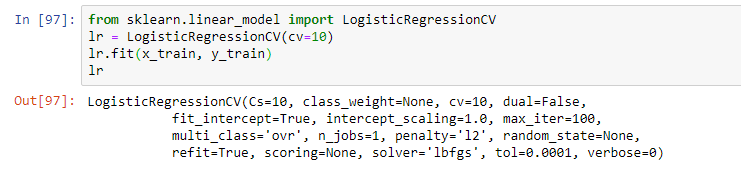
Next, select the model. As part of the webinar, the teacher proposed a simple logistic regression. The model was trained using the fit operation, which resulted in a model in the form of a logistic regression with certain parameters:
In practice, in practice, several models are usually used that seem to be the most effective. And the final solution is often a combination of these models with the help of stacking techniques and other approaches to the ensemble of models (using several models within one hybrid model).
After training, the model can be applied on test data, assessing its quality within a metric. In our case, the quality within accuracy_score was 0.8:
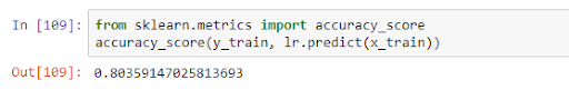
This means that on the received data the variable is correctly predicted in 80% of cases. Having obtained the learning results, we can either improve the model (if the accuracy is not satisfactory), or go directly to the forecast.
This was the end of the main topic of the lesson, but the teacher told in more detail about the features of using the model in different tasks and answered questions from the audience. So if you do not want to miss anything, watch the webinar completely if you are interested in this topic.
As always, we are waiting for your comments and questions that you can leave here or ask Alexander about them by visiting him on an open day.
In December, we will start training the next Data Scientist group , so there are more and more open lessons and other activities. For example, just recently, a webinar was held under the long title “Feature Engineering on the example of the classic Titanic dataset”. It was conducted by Alexander Sizov - an experienced developer, Ph.D., an expert on Machine / Deep learning and a participant in various commercial international projects related to artificial intelligence and data analysis.
Open lesson took about one and a half hours. During the webinar, the teacher spoke about the selection of signs, the transformation of the source data (coding, scaling), setting parameters, training the model and much more. In the course of the lesson, the participants were shown a Jupyter Notebook. Open source data from the Kaggle platform (a classic dataset about “Titanic”, from which many begin their acquaintance with Data Science) was used for work. Below we offer a video and transcript of the past event, and here you can pick up the presentation and codes in the Jupiter's laptop.
')
Feature selection
The topic was chosen, although classical, but still a bit gloomy. In particular, it was necessary to solve the problem of binary classification and predict according to the available data whether a passenger will survive or not. The data itself was divided into two samples, Training and Test. The key variable is Survival (survived / not survived; 0 = No, 1 = Yes).
Input training data:
- ticket class;
- age and sex of the passenger;
- marital status (are there any relatives on board);
- ticket price;
- cabin number;
- port of landing.
As you can see, the types of variables are different: numeric, text. From this kaleidoscope it was necessary to form a dataset for the upcoming training of the model.
We summarize:
- train.csv - training set - training data set. They know the answer - survival - binary sign 0 (did not survive) / 1 (survived);
- test.csv - test set - test data set. The answer is unknown. This is a sample to send to the kaggle platform to calculate the model quality metric;
- gender_submission.csv is an example of the format of the data that needs to be sent to kaggle.
Work algorithm
- The work took place in stages:
- Analyze data from train.csv.
- Handling missing values.
- Scaling.
- Coding categorical traits.
- Building a model and selecting parameters, choosing the best model on the converted data from train.csv.
- Fixation of the transformation method and model.
- Apply the same transformations on test.csv using the pipeline.
- Apply the model to test.csv.
- Saving to the file the results of the application in the same format as in gender_submission.csv.
- Sending results to the kaggle platform.
The practical part of the webinar
The first thing that needed to be done was to read the dataset and display our data on the screen:
For data analysis, a little-known but quite useful profiling library was used:
pandas_profiling.ProfileReport(df_train)Read more about profiling
This library does everything that can be done a priori without knowing the details about the data. For example, display statistics on data (how many variables and what type they are, how many lines, missing values, etc.). Moreover, separate statistics are given for each variable with the reduction of the minimum and maximum, the distribution graph, and other parameters.
As you know, in order to make a good model, you need to understand the process that we are trying to model and understand which features are key. And by no means always in our data there is everything that is needed, or, more precisely, almost never they lack all the necessary, fully determining and determining our process. As a rule, we always need to combine something, perhaps, to add additional features that are not represented in the dataset (say, the weather forecast). It is to understand the process and need data analysis, which can be done using the profiling library.
Missing values
The next step is to solve the problem of missing values, because in most cases the data is not completely filled.
There are the following solutions to this problem:
- delete rows with missing values (you need to consider that you can lose some important values);
- remove the sign (relevant if there is too little data on it);
- replace missing values with something else (median, average ...).
An example of a simple conversion using the fillna method, which assigns the values of the median variable to only those cells that are not filled:
In addition, the teacher showed examples of using Imputer and pipeline.
Feature scaling
The work of the model and the final decision depends on the scale of the signs. The fact is that it is not a fact that any sign, which has a larger scale, is more important than a sign, which has a smaller scale. That is why models need to submit attributes that are scaled in the same way, that is, having the same weight for the model.
There are different scaling techniques, but the format of the open lesson allowed us to consider in more detail only two of them:
Combinations of signs
Combinations of existing features using arithmetic operations (sum, multiplication, division) allow to obtain any feature that makes the model more efficient. This is not always possible, and we do not know which combination will give the desired effect, but practice shows that it makes sense to try. It is convenient to apply transformations of signs using the pipeline.
Coding
So, we have data of different types: numeric and text. Currently, most models on the market cannot work with textual data. As a result, all categorical features (textual) must be converted to a numerical representation, for which encoding is used.
Label encoding . This is the mechanism implemented in many libraries, which can be called and applied:
Label encoding assigns a unique identifier to each unique value. Minus - we bring order into some variable that was not ordered, which is not good.
OneHotEncoder. Unique text variable values are expanded as columns, which are added to the source data, where each column is a binary variable in the form of 0 and 1. This approach has no disadvantages of Label encoding, but has its own minus: if there are many unique values, we add too many columns and in some cases the method is simply not applicable (it increases too much).
Model training
After performing the above actions, a final pipeline is drawn up with a set of all necessary operations. Now it is enough to take the source dataset and apply the final pipeline on this data using the fit_transform operation:
x_train = vec.fit_transform(df_train)As a result, we get dataset x_train, which is ready for use in the model. The only thing that needs to be done is to separate the value of our target variable so that we can conduct the training.
Next, select the model. As part of the webinar, the teacher proposed a simple logistic regression. The model was trained using the fit operation, which resulted in a model in the form of a logistic regression with certain parameters:
In practice, in practice, several models are usually used that seem to be the most effective. And the final solution is often a combination of these models with the help of stacking techniques and other approaches to the ensemble of models (using several models within one hybrid model).
After training, the model can be applied on test data, assessing its quality within a metric. In our case, the quality within accuracy_score was 0.8:
This means that on the received data the variable is correctly predicted in 80% of cases. Having obtained the learning results, we can either improve the model (if the accuracy is not satisfactory), or go directly to the forecast.
This was the end of the main topic of the lesson, but the teacher told in more detail about the features of using the model in different tasks and answered questions from the audience. So if you do not want to miss anything, watch the webinar completely if you are interested in this topic.
As always, we are waiting for your comments and questions that you can leave here or ask Alexander about them by visiting him on an open day.
Source: https://habr.com/ru/post/433084/
All Articles