Need more different Blur's
Blurring an image using a Gaussian Blur filter is widely used in a variety of tasks. But sometimes you want a little more variety than just one filter for all occasions, in which only one parameter can be adjusted - its size. In this article, we will look at several other blur implementations.

The Gaussian Blur effect is a linear operation and is mathematically a convolution of an image with a filter matrix. In addition, each pixel in the image is replaced by the sum of nearby, taken with certain weight coefficients.
The filter is called Gaussian, because it is built from a function known as a Gaussian, :
')
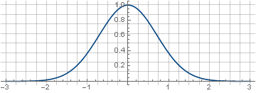
the two-dimensional version of which is obtained by its rotation about the ordinate axis, :
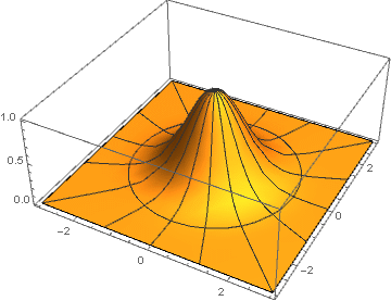
Here for each pair of coordinates the distance to the center is calculated by the formula which is passed as an argument to the function of the Gaussian - and, as is easy to see, reduced to .
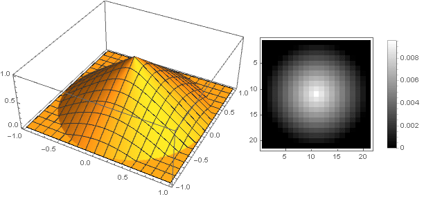
Matrix built on a segment and with some level of discretization, it will look like this:
Or, if we consider the values of the matrix elements as the brightness level, so:
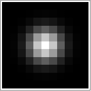
In terms of signal processing, this is called impulse response, since this is exactly what the result of the convolution of a given filter with a single pulse (in this case, a pixel) will look like.
Initially, a Gaussian is defined on an infinite interval. But due to the fact that it rather quickly fades away, it is possible to exclude values close to zero from the calculations, since they will not affect the result anyway. In real-world applications, normalization by value is also necessary so that after convolution the image brightness does not change; and in the case of blurring an image in which each pixel has the same color, the image itself should not change.
For convenience, the normalization is often used along the coordinates, by introducing an additional parameter (reads "sigma") - to treat an argument in the range , but determines the degree of compression of the Gaussians:
Normalizing divider here obtained analytically through a definite integral at infinity:
Due to the equality , the Gauss blur can be implemented sequentially, first in rows and then in columns - which allows you to save quite a lot on calculations. In this case, it is necessary to use the formula with normalization for the one-dimensional case -
For an arbitrary filter, we first need to define our own decay function for one variable. from which a function of two variables is obtained by rotation by replacing on where and these are the coordinates of the matrix element in the range , and which is further used to fill the elements of the matrix. We will consider normalization not analytically, but direct summation of all elements of the matrix — this is simpler and more accurate — because after sampling the function is “thinned”, and the normalization value will depend on the level of discretization.
If the matrix elements are numbered from zero, the coordinate or is calculated by the formula
Where - the sequence number of the element in the row or column, and - total number of items.
For example, for a 5 by 5 matrix, it would look like this:
Or, if we exclude the boundary values that are still zero, then the coordinates will be calculated by the formula
and the matrix, respectively, takes the form
After the matrix elements have been calculated by the formula, it is necessary to calculate their sum and divide the matrix into it. For example, if we have a matrix
then the sum of all its elements will be 40, and after normalization it will take the form
and the sum of all its elements will be 1.
First, take the simplest function - the line:
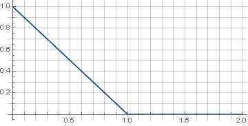
Piecewise-continuous definition here requires that the function is guaranteed to go to zero and during rotation there are no artifacts at the corners of the matrix. In addition, since the rotation uses the root of the sum of squares of coordinates, which is always positive, it is sufficient to determine the function only in the positive part of the values. As a result, we get:
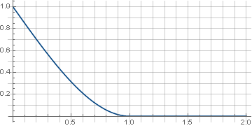
The abrupt transition from a sloping line to zero functions can cause a contradiction with a sense of beauty. The function will help us to eliminate it.
wherein defines the “hardness” of the docking, . For example will get
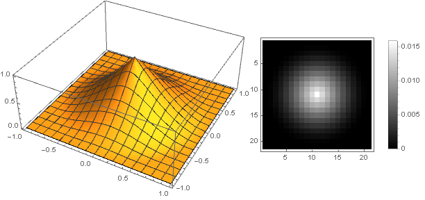
and the filter itself will look like
The filter can be made more “sharp” and more smoothly going to zero, taking another function as a generator, for example, hyperbola, and providing a smooth transition to zero by summing with a parabola.
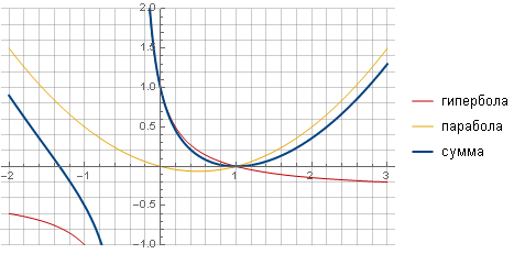
After all the calculations and simplifications, we obtain the formula
in which parameter determines the nature of the attenuation:
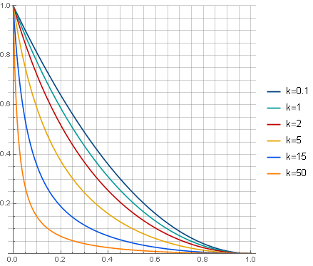
and the filter itself will look (for ) as

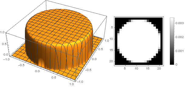
You can go the other way - to make the top of the filter is not sharp, but stupid. The easiest way to do this is to set the attenuation function as a constant:
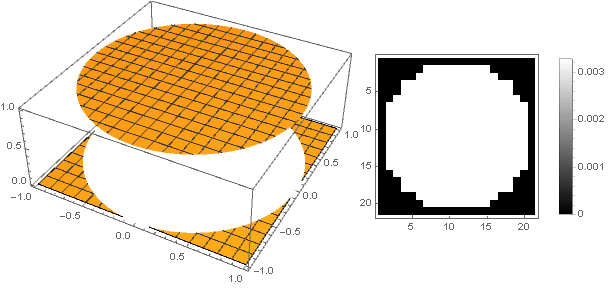
But in this case we get a strong pixelation, which contrasts with the sense of beauty. To make it smoother at the edges, a parabola of higher orders will help us, from which by its displacement along the ordinate axis and squaring we get
Varying the parameter You can get a wide range of filter options:
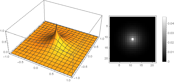

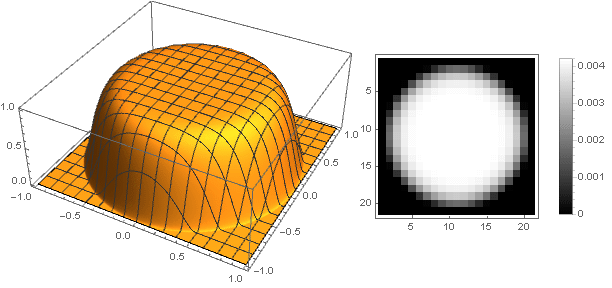
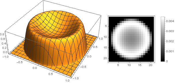
And slightly modifying the attenuation function, you can make a more pronounced ring at the edges of the filter, for example:
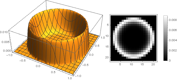
Here is the parameter determines the height of the center, and - the sharpness of the transition to the edges.
For will get
and for
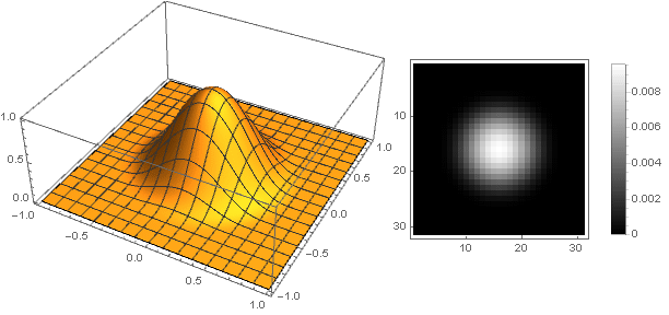
You can modify directly the function of the Gaussians. The most obvious way to do this is to parameterize the exponent — we are not going to consider it now, but take a more interesting option:
Due to the fact that tending to unit denominator tends to zero fraction tends to minus infinity, and the exponent itself also tends to zero. Thus, the division by allows you to compress the domain of a function with before . At the same time, with by dividing by zero ( ) the value of the function is not defined, but it has two limits - the limit on the one hand (from the inside) is zero, and on the other hand - infinity:
Since the boundary values are not included in the interval, then zero in the limit on one side only is sufficient. Interestingly, this property extends to all derivatives of this function, which provides an ideal connection with zero.
Parameter determines the similarity with the Gaussian - the more it is, the stronger the similarity is obtained - due to the fact that an increasingly linear segment fall at the center of the function. One would assume that due to this in the limit one can get the original Gaussian - but, unfortunately, no - the functions are still different.

Now you can see what happened:
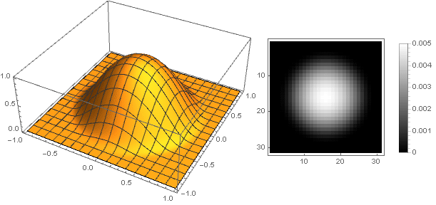
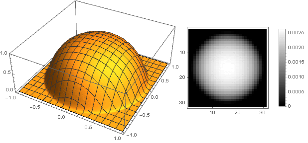
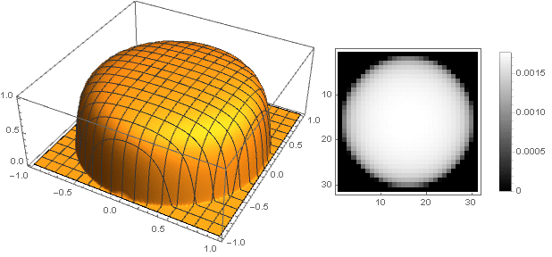

Changing the transition function from two coordinates to one , you can get other shapes, not just a disk. For example:
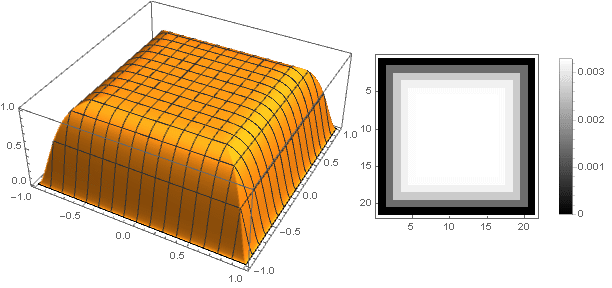
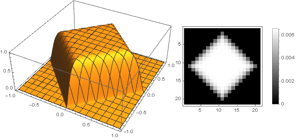
Turning to complex numbers, you can construct more complex shapes:
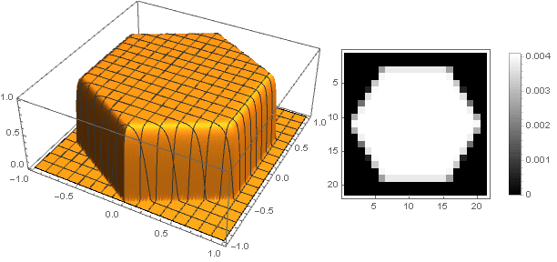
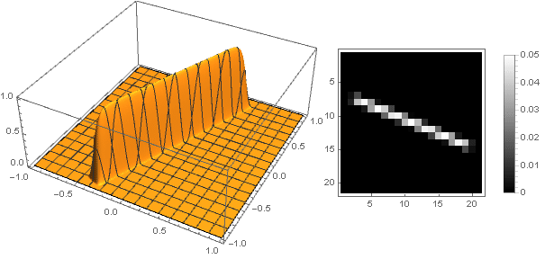
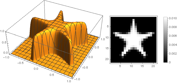
At the same time, it is necessary to ensure that when converting coordinates not to go beyond the interval - well, or vice versa, to define the damping function for negative values of the argument.
An article would not be complete without practical testing on specific images. Since we don’t have a scientific work, we won’t take Lena’s image, but take something soft and fluffy:


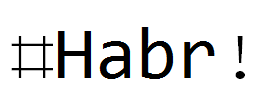
Same filters, but for text:


Similarly, you can build more complex filters, including with sharpening or contouring; as well as modify the already considered.
Of particular interest is nonlinear filtering, when the values of the filter coefficients depend on the coordinates or the directly filtered image itself - but this is a subject for other studies.
In more detail, the derivation of functions for docking with a constant is discussed here . As a damping function, the window functions discussed here can also be used — all that is needed is to scale the argument c (0,1) to ( , 1) or initially consider window functions by the formula .
The original Wolfram Mathematica document for this article can be downloaded here .

Introduction
The Gaussian Blur effect is a linear operation and is mathematically a convolution of an image with a filter matrix. In addition, each pixel in the image is replaced by the sum of nearby, taken with certain weight coefficients.
The filter is called Gaussian, because it is built from a function known as a Gaussian, :
')

the two-dimensional version of which is obtained by its rotation about the ordinate axis, :

Here for each pair of coordinates the distance to the center is calculated by the formula which is passed as an argument to the function of the Gaussian - and, as is easy to see, reduced to .
Matrix built on a segment and with some level of discretization, it will look like this:
Or, if we consider the values of the matrix elements as the brightness level, so:

In terms of signal processing, this is called impulse response, since this is exactly what the result of the convolution of a given filter with a single pulse (in this case, a pixel) will look like.
Initially, a Gaussian is defined on an infinite interval. But due to the fact that it rather quickly fades away, it is possible to exclude values close to zero from the calculations, since they will not affect the result anyway. In real-world applications, normalization by value is also necessary so that after convolution the image brightness does not change; and in the case of blurring an image in which each pixel has the same color, the image itself should not change.
For convenience, the normalization is often used along the coordinates, by introducing an additional parameter (reads "sigma") - to treat an argument in the range , but determines the degree of compression of the Gaussians:
Normalizing divider here obtained analytically through a definite integral at infinity:
Due to the equality , the Gauss blur can be implemented sequentially, first in rows and then in columns - which allows you to save quite a lot on calculations. In this case, it is necessary to use the formula with normalization for the one-dimensional case -
Start
For an arbitrary filter, we first need to define our own decay function for one variable. from which a function of two variables is obtained by rotation by replacing on where and these are the coordinates of the matrix element in the range , and which is further used to fill the elements of the matrix. We will consider normalization not analytically, but direct summation of all elements of the matrix — this is simpler and more accurate — because after sampling the function is “thinned”, and the normalization value will depend on the level of discretization.
If the matrix elements are numbered from zero, the coordinate or is calculated by the formula
Where - the sequence number of the element in the row or column, and - total number of items.
For example, for a 5 by 5 matrix, it would look like this:
Or, if we exclude the boundary values that are still zero, then the coordinates will be calculated by the formula
and the matrix, respectively, takes the form
After the matrix elements have been calculated by the formula, it is necessary to calculate their sum and divide the matrix into it. For example, if we have a matrix
then the sum of all its elements will be 40, and after normalization it will take the form
and the sum of all its elements will be 1.
Linear attenuation
First, take the simplest function - the line:

Piecewise-continuous definition here requires that the function is guaranteed to go to zero and during rotation there are no artifacts at the corners of the matrix. In addition, since the rotation uses the root of the sum of squares of coordinates, which is always positive, it is sufficient to determine the function only in the positive part of the values. As a result, we get:

Soft linear attenuation
The abrupt transition from a sloping line to zero functions can cause a contradiction with a sense of beauty. The function will help us to eliminate it.
wherein defines the “hardness” of the docking, . For example will get

and the filter itself will look like

Hyperbolic attenuation
The filter can be made more “sharp” and more smoothly going to zero, taking another function as a generator, for example, hyperbola, and providing a smooth transition to zero by summing with a parabola.

After all the calculations and simplifications, we obtain the formula
in which parameter determines the nature of the attenuation:

and the filter itself will look (for ) as

Bokeh effect imitation
You can go the other way - to make the top of the filter is not sharp, but stupid. The easiest way to do this is to set the attenuation function as a constant:

But in this case we get a strong pixelation, which contrasts with the sense of beauty. To make it smoother at the edges, a parabola of higher orders will help us, from which by its displacement along the ordinate axis and squaring we get
Varying the parameter You can get a wide range of filter options:


And slightly modifying the attenuation function, you can make a more pronounced ring at the edges of the filter, for example:
Here is the parameter determines the height of the center, and - the sharpness of the transition to the edges.
For will get

and for

Variations of Gaussians
You can modify directly the function of the Gaussians. The most obvious way to do this is to parameterize the exponent — we are not going to consider it now, but take a more interesting option:
Due to the fact that tending to unit denominator tends to zero fraction tends to minus infinity, and the exponent itself also tends to zero. Thus, the division by allows you to compress the domain of a function with before . At the same time, with by dividing by zero ( ) the value of the function is not defined, but it has two limits - the limit on the one hand (from the inside) is zero, and on the other hand - infinity:
Since the boundary values are not included in the interval, then zero in the limit on one side only is sufficient. Interestingly, this property extends to all derivatives of this function, which provides an ideal connection with zero.
Parameter determines the similarity with the Gaussian - the more it is, the stronger the similarity is obtained - due to the fact that an increasingly linear segment fall at the center of the function. One would assume that due to this in the limit one can get the original Gaussian - but, unfortunately, no - the functions are still different.

Now you can see what happened:


Form variations
Changing the transition function from two coordinates to one , you can get other shapes, not just a disk. For example:


Turning to complex numbers, you can construct more complex shapes:


At the same time, it is necessary to ensure that when converting coordinates not to go beyond the interval - well, or vice versa, to define the damping function for negative values of the argument.
Some specific examples
An article would not be complete without practical testing on specific images. Since we don’t have a scientific work, we won’t take Lena’s image, but take something soft and fluffy:

Gaussiana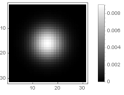


Hyperbolic attenuation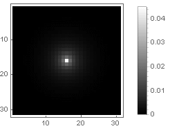


Cross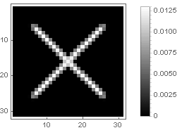


Ring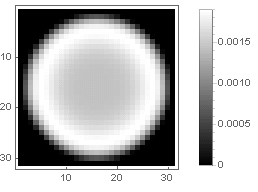


One-way attenuation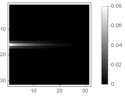


Same filters, but for text:


Conclusion
Similarly, you can build more complex filters, including with sharpening or contouring; as well as modify the already considered.
Of particular interest is nonlinear filtering, when the values of the filter coefficients depend on the coordinates or the directly filtered image itself - but this is a subject for other studies.
In more detail, the derivation of functions for docking with a constant is discussed here . As a damping function, the window functions discussed here can also be used — all that is needed is to scale the argument c (0,1) to ( , 1) or initially consider window functions by the formula .
The original Wolfram Mathematica document for this article can be downloaded here .
Source: https://habr.com/ru/post/432622/
All Articles