How to forecast demand and automate purchases using machine learning: Ozon case

In the online store Ozon there is just about everything: refrigerators, baby food, laptops for 100 thousand, etc. It means that all this is in the company's warehouses - and the longer the goods are there, the more expensive the company is. To find out how much and what people want to order, and Ozon will need to be purchased, we used machine learning.
Sales forecast: challenges
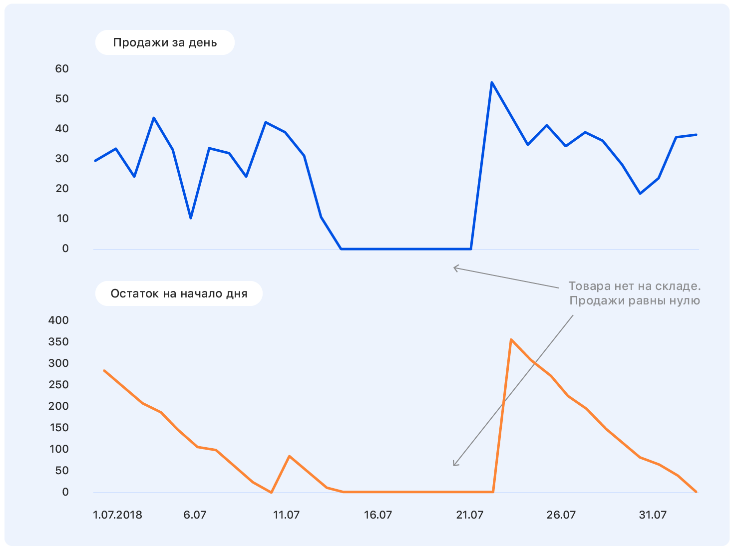
Before we delve into the formulation of the problem, we begin with an example. This is a real schedule of sales of goods on Ozon for some time. Question: where will he go next?
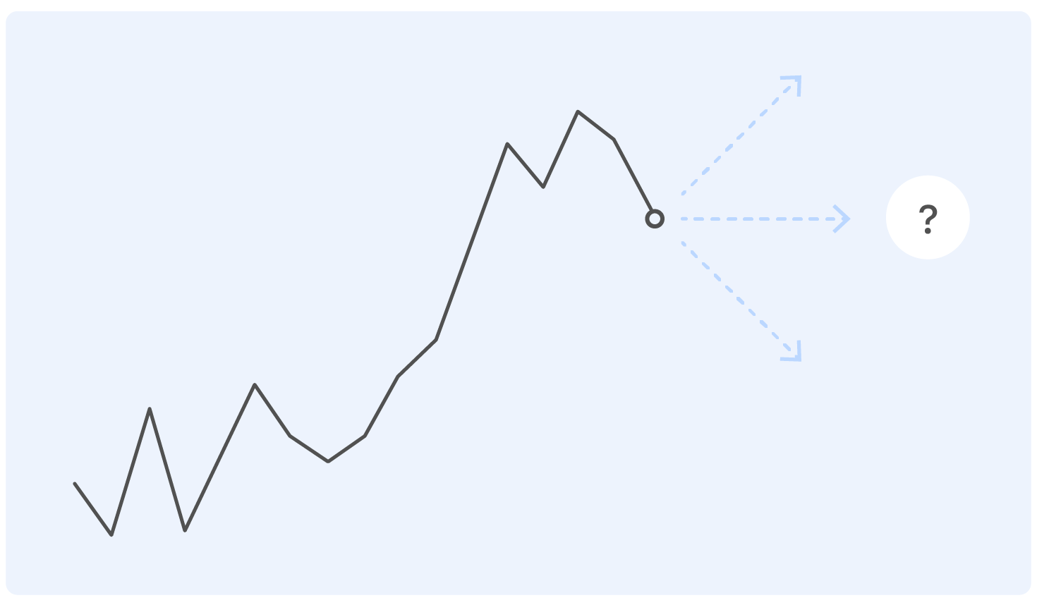
A person with a near-technical education to this formulation of the problem will have questions: And where are the axes? And what kind of product? And in what units? What institute graduated from? - and many others not included in this article for ethical reasons.
')
In fact, no one can answer the question correctly in such a statement, and if someone can, he is most likely mistaken.
Add some more information to this graphic: axles and price changes on the Ozon website (blue) and on the competitor's website (orange).
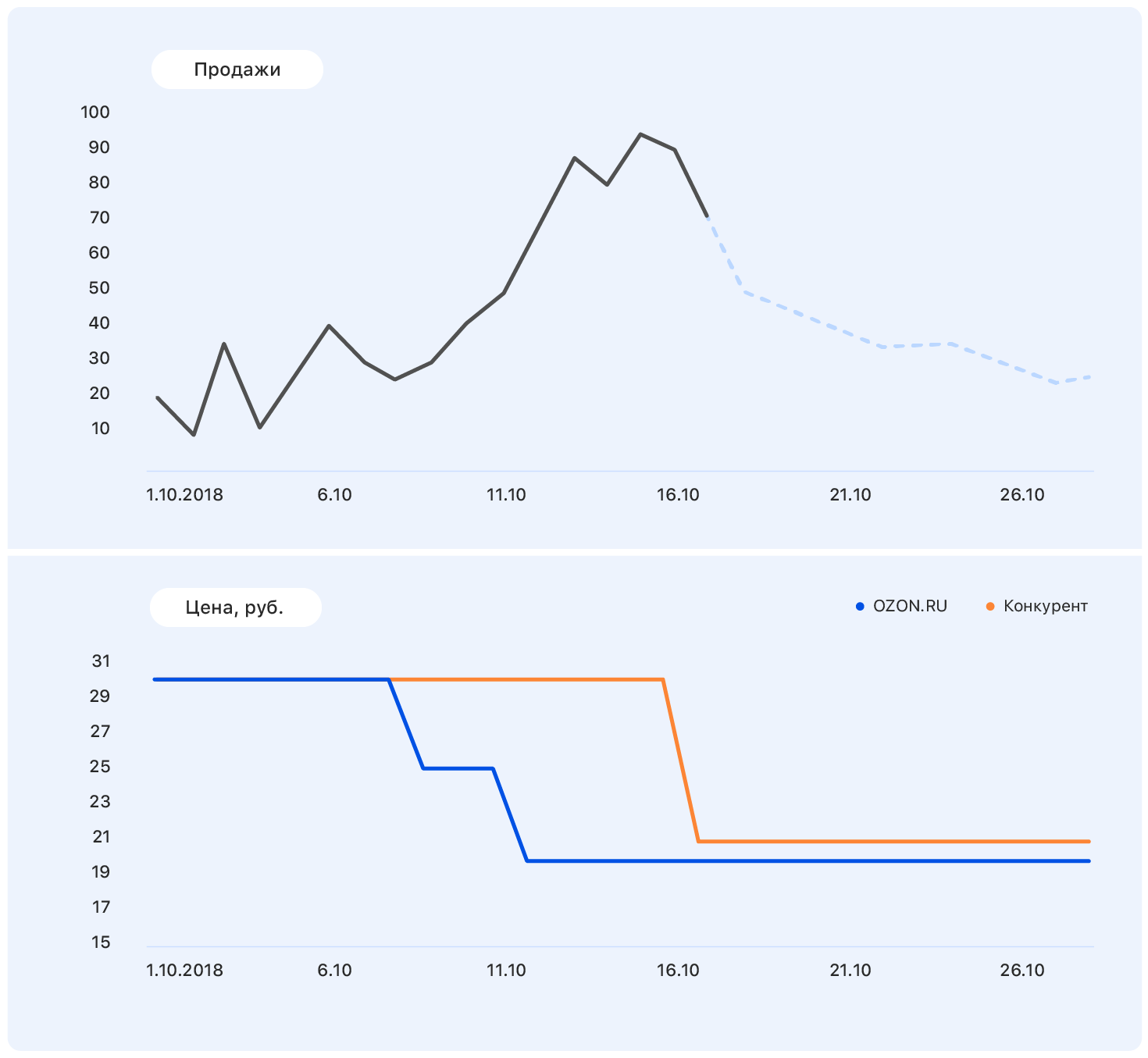
At some point, the price at our place has decreased, while the competitors have remained the same - and sales at Ozon have gone up. We know pricing plans: our price will remain at the same level, but the competitor, following Ozon, lowered the price to almost ours.
This data is enough to make a sensible assumption - for example, that sales will return to their previous level. And if you look at the chart, it turns out that it will be so.
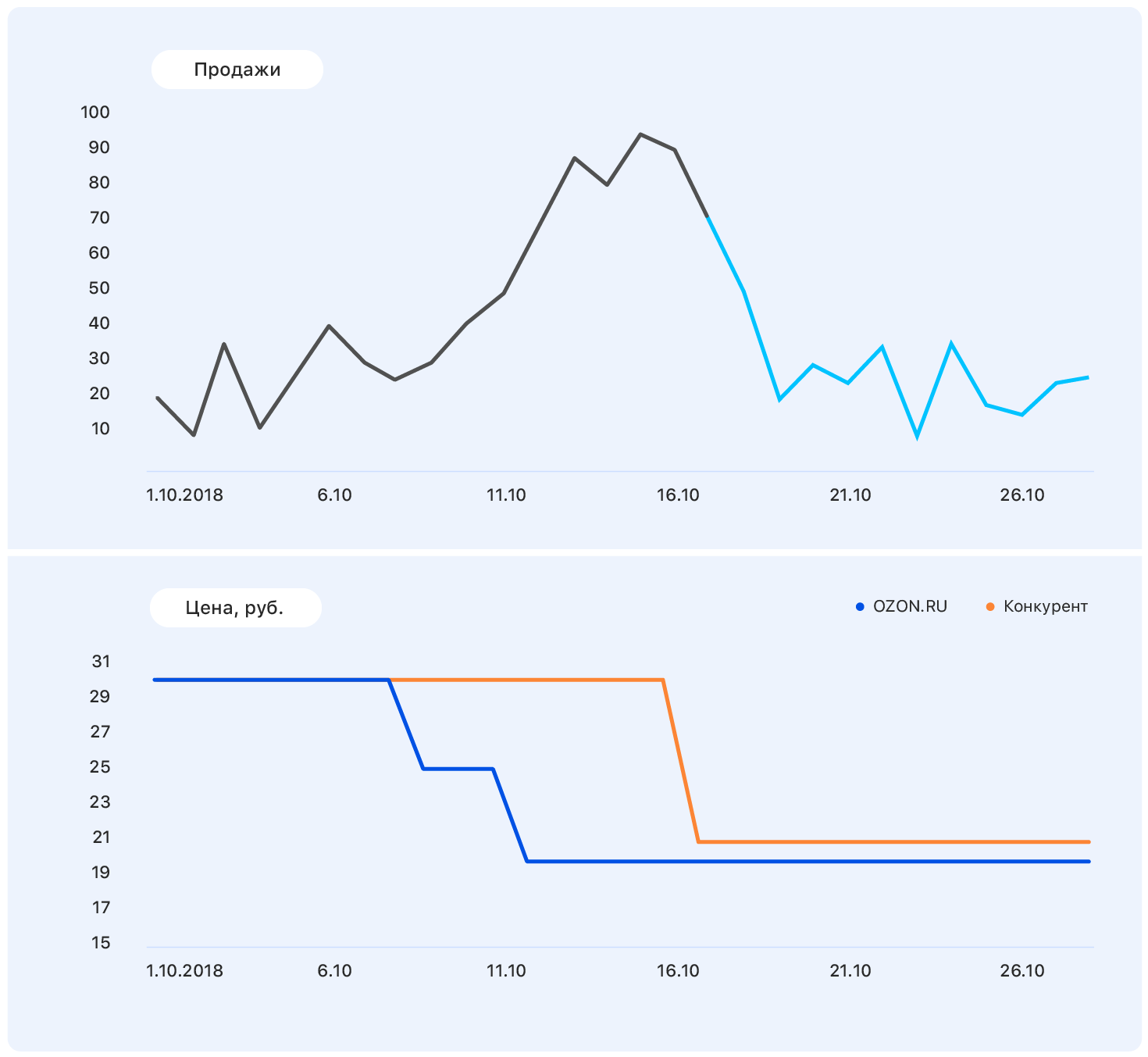
The problem is that in fact the demand for this product is not so much affected by the price, and sales growth was caused, among other things, by the absence of most of the competitors of this product in our store. There are still many factors that we did not take into account: was the product advertised on TV? or maybe it's candy, and soon March 8?
One thing is clear: make a forecast "on the knee" will not work. We went along the standard path of the
Metric selection
Choosing a metric is where to start if your forecast will be used by at least one other person besides you.
Consider an example: we have three projections. Which is better?
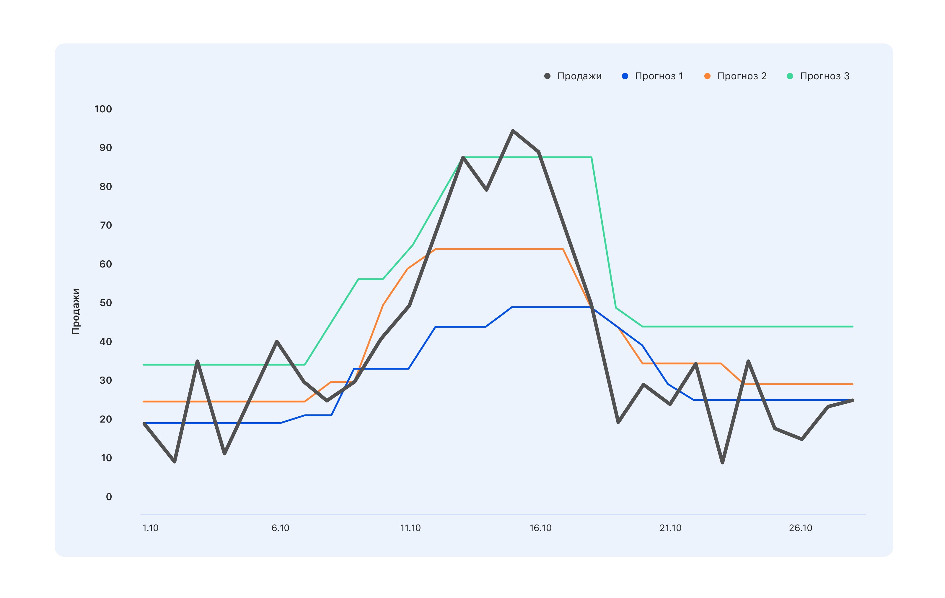
From the point of view of specialists in the warehouse, we need a blue forecast - buy a little less, and let us miss the peak in mid-October, but nothing is left in the warehouse. The experts, whose KPI are tied to sales, have the opposite opinion: even the turquoise forecast is not quite correct, not all demand spikes reflected - go and modify. And from the point of view of a person from the outside, something in between is generally better - so that everyone is good, or vice versa bad.
Therefore, before building a forecast, it is necessary to determine who will use it and why. That is, choose a metric and understand what to expect from the forecast based on such a metric. And wait for just that.
We chose MAE - the average absolute error. This metric is suitable for our highly unbalanced training set. Since the range is very wide (1.5 million items), each product individually in a particular region is sold in small quantities. And if in total we sell hundreds of green dresses, then a particular green dress with cats sells for 2-3 per day. As a result, the sample is shifted towards small values. On the other hand, there are iPhones, spinners, a new book by Olga Buzova (joke), etc. - and they are sold in any city in large quantities. MAE allows you not to receive huge fines on conditional iPhones and generally work well on the bulk of the goods.
The first steps
We began by building the stupidest prediction that could be: a random number from 0 to 1000 will be sold over the next week - and we got the metric MAE = 496. Probably, it can be worse, but this is already very bad. So we got a guideline: if we get such a metric value, then obviously we are doing something wrong.
Then we started to play people who know how to make a forecast without machine learning, and tried to predict the sale of goods for the next week equal to the average sales for all the past weeks, and received the MAE metric = 1.45 - which is much better.
Continuing to argue, we decided that the more relevant for the forecast of sales for the next week would not be the average, but sales for the last week. In this forecast, MAE was equal to 1.26. In the next round of predictive thinking, we decided to take both factors into account and predict sales for the next week as the sum of 50% of average sales and 50% of sales over the last week - we received MAE = 1.23.
But this seemed too simple to us, and we decided to make everything more complicated. We collected a small training sample in which the signs were past and average sales, and the targets were sales for the next week, and we trained on it a simple linear regression. We obtained weights of 0.46 and 0.55 for the average and last weeks and MAE on the test sample, equal to 1.2.
Conclusion: our data has a prognostic potential.
Feature engineering
Deciding that building a forecast on two grounds is not our level, we sat down to generate new complex features. This and information about past sales - for 1, 2, 3, 4 weeks ago, a week exactly a year ago, etc. And views over the past weeks, adding to the cart, converting views and adding to the cart in orders - and all this for different periods.
We needed to give the model knowledge of how the product as a whole is sold, how the dynamics of its sales has changed recently, how interest in it evolves, how its sales depend on price and other factors that we think can be useful.
When our ideas ran out, we went to the sales department experts. There, for example, we learned that the next year is the year of the pig, therefore goods, even remotely resembling pigs, will enjoy increased popularity. Or, for example, that our people do not buy the “freeze-up” in advance, but on the very day of the first frost - so please, take into account the weather forecast. In general, everyone was happy. We have got a lot of new ideas that we would never have thought of ourselves, and merchants that we can soon be doing something more interesting than the sales forecast.
But it is still too simple - and we added combined features:
- conversion from views to sales - what it was, how it changed;
- the ratio of sales for 4 weeks to sales for the last week (if this figure is very different from 4, at the moment the demand for this product is subject to "turbulence");
- the ratio of sales of goods to sales in the whole category - if this figure is close to one, then the product is a “monopolist”.
At this stage, you need to come up with as much as possible - throw out non-informative signs at the training stage.
As a result, we got 170 signs. Looking ahead, the greatest
- Sales last week (for two, three and four).
- The availability of the product last week - the percentage of time when the product was present on the site.
- Angular coefficient of the sales schedule for the last 7 days.
- The ratio of past price to future - with a huge discount to start buying goods more actively.
- The number of direct competitors within our site. If, for example, this pen is unique in its category, sales will be fairly stationary.
- The dimensions of the product - it turned out that the length and width significantly affect the predictability of sales. For some reason, for long and narrow objects - umbrellas or fishing rods, for example - the schedule is much more volatile. We do not yet know how to explain it.
- The number of the day in the year - it shows whether the New Year is coming soon, March 8, the start of a seasonal increase in sales, etc.
Sampling collection
Teaching sample is pain. We collected it for about 4 weeks, two of which simply went to different data keepers and asked to see what they have. This happens every time you need data for a long period. Even in an ideal data collection system, something like this would happen in a long time, “we used to think this thing like this, but then we started to think differently and write data in the same column.” Or a year or two ago the server fell, but no one recorded exactly when - and the zeros no longer mean that there was no sales.
As a result, we had at our disposal information about what people were doing on the site, what they added to their favorites and the basket, and how much they bought. We collected a sample of about 15 million samples of 170 features each, the target was the number of sales for the next week.
We wrote 2 thousand lines of code on Spark. He worked slowly, but allowed to chew through huge amounts of data. It only seems that to calculate the angular coefficient of a straight line is simple. And to do this 10kk times, when sales are drawn from several bases - the task is not for the faint of heart.
For another week, we cleaned the data so that the model was not distracted by outliers and local sampling features, but extracted only the true dependencies inherent in Ozon sales. Here will go both 3 sigma and more cunning methods of search for anomalies. The most difficult case is to restore sales during periods when the product is out of stock. The simplest solution is to throw away the weeks when the product was absent during the “targeted” week.
As a result, 10 million of 15 million samples remained. Here it is important not to get carried away and not lose the completeness of the sample (in fact, the lack of goods in the warehouse is an indirect characteristic of its importance for the company; to remove such products from the sample is not the same as throwing random samples ).
ML time
On a clean sample and began to train the model. Naturally, we started with linear regression and got MAE = 1.15. It seems that this is a very small increase, but when you have a sample of 10 million in which the average values are 5-10, even a small change in the value of the metric gives a disproportionate increase in the visual quality of the forecast. And since in the end you will have to present the solution to business customers, raising their level of joy is an important factor.
Next was sklearn.ensemble.RandomForestRegressor, which after a short selection of hyper parameters showed MAE = 1.10. Next we tried XGBoost (where without it) - everything would be fine and MAE = 1.03 - only for a very long time. Unfortunately, we did not have access to the GPU for learning XGBoost, and on the processors one model was trained for a very long time. We tried to find something faster, and stopped at LightGBM - he studied twice as fast and showed MAE even a little less - 1.01.
We have broken all products into 13 categories, just like in the catalog on the site: tables, laptops, bottles, and for each of the categories we trained models with different depths of the forecast - from 5 to 16 days.
The training took about five days, and for this we raised huge computing clusters. We have developed such a pipeline: random search works for a long time, gives the top 10 sets of hyperparameters, and then the scientist works the date with them manually - builds additional quality metrics (we considered MAE for different ranges of targets), builds learning curves (for example, we threw out some of the training sampling and trained again, checking whether new data reduces loss on the test sample) and other graphs.
An example of a detailed analysis for one of the sets of hyperparameters:
Detailed quality metric
Train loss = 0.535842111392
Test loss = 0.895529959873
Train set: | Test set: |
| For target = 0, MAE = 0.142222484602 | For 0 MAE = 0.141900737761 |
| For target> 0 MAPE = 45.168530676 | For> 0, MAPE = 45.5771812826 |
| More errors than 0 - 67.931341691% | More errors 0 - 51.6405939896% |
| Errors greater than 1 - 19.0346986379% | Errors greater than 1 - 12.1977096603% |
| Errors greater than 2 - 8.94313926245% | Errors greater than 2 - 5.16977226441% |
| Errors greater than 3 - 5.42406856507% | Errors greater than 3 - 3.12760834969% |
| More than 4 errors - 3.67938161595% | More than 4 errors - 2.10263125679% |
| More than 5 errors - 2.67322988948% | More than 5 errors - 1.56473158807% |
| More than 6 errors - 2.0618556701% | More than 6 errors - 1.19599209102% |
| More than 7 errors - 1.65887701209% | More than 7 errors - 0.949300173983% |
| There are more than 8 errors - 1.36821095777% | More than 8 errors - 0.78310772461% |
| More than 9 errors - 1.15368611519% | More than 9 errors - 0.659205318158% |
| More than 10 errors - 0.99199395014% | More than 10 errors - 0.554593106723% |
| More errors than 11 - 0.863969667827% | More errors than 11 - 0.490045146476% |
| There are more than 12 errors - 0.764347266082% | There are more than 12 errors - 0.428835873827% |
| More than 13 errors - 0.68086818247% | Errors greater than 13 - 0.386545830907% |
| More than 14 errors - 0.613446089087% | More than 14 errors - 0.343884822697% |
| More than 15 errors - 0.556297016335% | There are more than 15 errors - 0.316433391328% |
| For target = 0, MAE = 0.142222484602 | For target = 0, MAE = 0.141900737761 |
| For target = 1, MAE = 0.63978556493 | For target = 1, MAE = 0.660823509405 |
| For target = 2, MAE = 1.01528075312 | For target = 2, MAE = 1.01098070566 |
| For target = 3, MAE = 1.43762342295 | For target = 3, MAE = 1.44836233499 |
| For target = 4, MAE = 1.82790678437 | For target = 4, MAE = 1.86539223382 |
| For target = 5, MAE = 2.15369976552 | For target = 5, MAE = 2.16017884573 |
| For target = 6, MAE = 2.51629758129 | For target = 6, MAE = 2.51987403661 |
| For target = 7, MAE = 2.80225497415 | For target = 7, MAE = 2.97580015564 |
| For target = 8, MAE = 3.09405048248 | For target = 8, MAE = 3.21914648525 |
| For target = 9, MAE = 3.39256765159 | For target = 9, MAE = 3.54572928241 |
| For target = 10, MAE = 3.6640339953 | For target = 10, MAE = 3.84409605282 |
| For target = 11, MAE = 4.02797747118 | For target = 11, MAE = 4.21828735273 |
| For target = 12, MAE = 4.17163467899 | For target = 12, MAE = 3.92536509115 |
| For target = 14, MAE = 4.78590364522 | For target = 14, MAE = 5.11290428675 |
| For target = 15, MAE = 4.89409916994 | For target = 15, MAE = 5.20892023117 |
Train loss = 0.535842111392
Test loss = 0.895529959873
Graph prediction (target) for the training sample
Graph prediction (target) for the test sample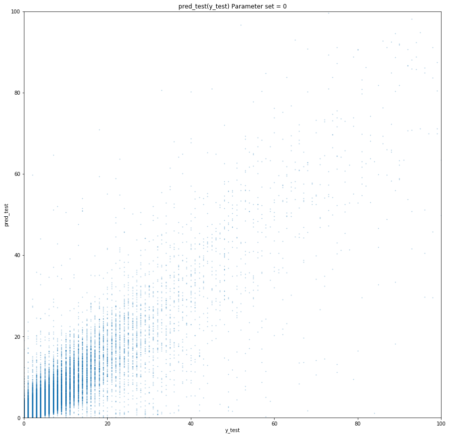
Prediction error from time to time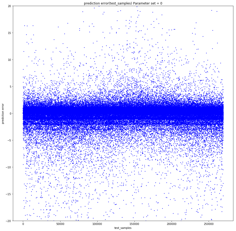
Sorted in ascending error on the test sample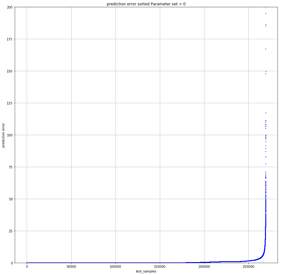
If none is suitable - again random search. This is how we trained a model for five or four days at an industrial rate. We were on duty, someone at night, someone woke up in the morning, looked at the top 10 parameters, restarted or saved the model, and went to sleep. In this mode, we worked for a week and trained 130 models - 13 types of goods and 10 forecast depths, each had 170 features. The average MAE value for a 5-fold time series cv was equal to 1.
It may seem that this is not very cool - and this is true, if only you have not a large part of the sample in the sample. As the analysis of the results shows, the units are predicted worst of all - the fact that a product bought once a week does not say whether there is a demand for it. One time, anything can be sold - there is a person who buys a porcelain figurine in the form of a dentist, and this does not say anything about future sales or about the past. In general, we did not get very upset about this.
Tips and tricks
What went wrong and how can you avoid it?
The first problem is the selection of parameters. We started using RandomizedSearchCV - this is the famous sklearn tool for iterating over hyper parameters. This is where the first surprise awaited us.
Like this
from sklearn.model_selection import ParameterSampler
from sklearn.model_selection import RandomizedSearchCV

estimator = lightgbm.LGBMRegressor(application='regression_l1', is_training_metric = True, objective = 'regression_l1', num_threads=72)
param_grid = {'boosting_type': boosting_type, 'num_leaves': num_leaves, 'max_depth': max_depth, 'learning_rate':learning_rate, 'n_estimators': n_estimators, 'subsample_for_bin': subsample_for_bin, 'min_child_samples': min_child_samples, 'colsample_bytree': colsample_bytree, 'reg_alpha': reg_alpha, 'max_bin': max_bin}

rscv = RandomizedSearchCV(estimator, param_grid, refit=False, n_iter=100, scoring='neg_mean_absolute_error', n_jobs=1, cv=10, verbose=3, pre_dispatch='1*n_jobs', error_score=-1, return_train_score='warn')

rscv .fit(X_train.values, y_train['target'].values)
print('Best parameters found by grid search are:', rscv.best_params_)
The calculation simply stalls (which is important, it does not fall, but continues to work, but at an ever smaller number of cores and at some point simply stops).
I had to parallelize the process by RandomizedSearchCV
estimator = lightgbm.LGBMRegressor(application='regression_l1', is_training_metric = True, objective = 'regression_l1', num_threads=1)

rscv = RandomizedSearchCV(estimator, param_grid, refit=False, n_iter=100, scoring='neg_mean_absolute_error', n_jobs=72, cv=10, verbose=3, pre_dispatch='1*n_jobs', error_score=-1, return_train_score='warn')

rscv .fit(X_train.values, y_train['target'].values)
print('Best parameters found by grid search are:', rscv.best_params_)
But RandomizedSearchCV for every job, almost the entire datas rambles. Accordingly, it is necessary to greatly expand the amount of RAM, perhaps sacrificing the number of cores.
Who would tell us then about such beautiful things as hyperopt! Since we learned, we only use it.
Another trick that came to our mind closer to the end of the project was to choose models that had the colsample_bytree parameter (this is the LightGBM parameter that says what percentage of features to give to each lerner) around 0.2-0.3, because when the machine It works in production, some tables may not exist, and individual features may not be calculated correctly. Such a regularization allows us to make these uncalculated features affect at least not all Lerners within the model.
Empirically, we came to the conclusion that we need to do more estimators and tighten the regularization more strongly. This is not the rule for working with LightGBM, but this scheme worked for us.
And, of course, Spark. For example, there is a bug that Spark himself knows: if you take several columns from a table and make a new one, and then take another one from the same table and make a new one, and then bake the resulting tables, everything will break, although it should not. You can escape only by getting rid of all the lazy calculations. We even wrote a special function - bumb_df, it turns the Data Frame into an RDD back into a Data Frame. That is, resets all lazy calculations. This can protect yourself against most Spark problems.
bumb_df
def bump_df(df):
# to avoid problem: AnalysisException: resolved attribute(s)
df_rdd = df.rdd
if df_rdd.isEmpty():
df = df_rdd.toDF(schema=df.schema)
return df
else:
return df_rdd.toDF(schema=df.schema)
The forecast is ready: how much will we order?
The sales forecast is a purely mathematical task, and if the normal distribution of an error with a zero average for a mathematician is a victory, then for merchants who have every ruble in their account is unacceptable.
If one extra iPhone or one fashionable dress in the warehouse is not a problem, but rather an insurance stock, then the absence of the same iPhone in the warehouse is a loss of at least margin, and as a maximum - an image, and this cannot be allowed.
To teach the algorithm to buy as much as necessary, we had to calculate the cost of over- and under-purchasing each product and train a simple model to minimize possible losses in money.
The model receives a sales forecast at the input, adds random, normally distributed noise to it (we simulate the imperfection of suppliers) and learns to add only enough to the forecast for each particular product in order to minimize money losses.
Thus, an order is a forecast + safety stock guaranteeing coverage of the error of the forecast itself and the nonideality of the outside world.
As in the sale
Ozon has its own rather large computing cluster, on which the pipeline starts every night (we use airflow) from more than 15 jobs. It looks like this:
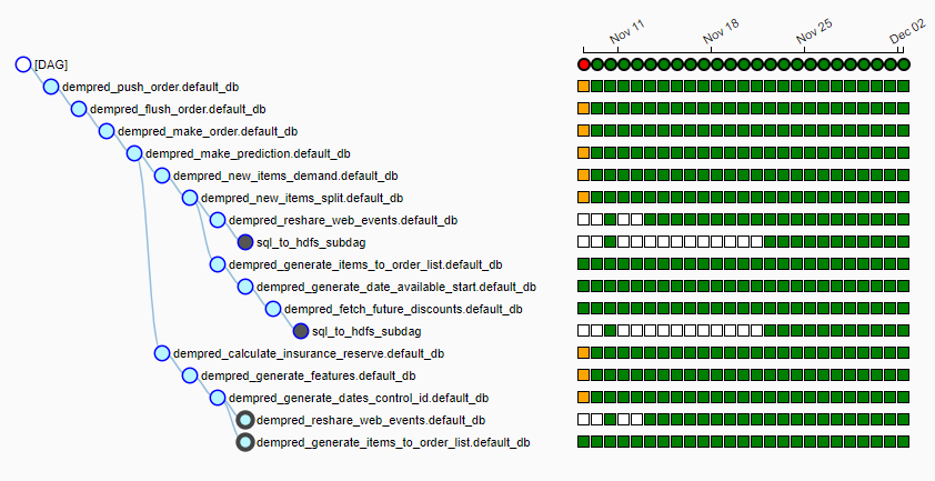
Every night, the algorithm runs, delays in local hdfs about 20 GB of data from various sources, selects a supplier for each product, collects features for each product, makes a sales forecast and generates bids based on the delivery schedule. By 6-7 in the morning we give the table to the people who are responsible for working with suppliers, ready-made tables, which at the touch of a button fly away to the suppliers.
Not a single forecast
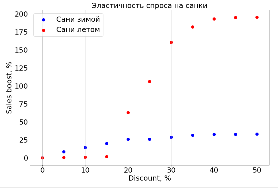
The trained model is aware of the dependence of the forecast on any feature and, as a result, if you freeze the N-1 signs and start changing one, you can observe how it affects the forecast. Of course, the most interesting thing about this is how sales depend on price.
It is important to note that demand depends not only on price. For example, if in the summer to make small discounts on the sled, it still does not help them sell. We make a discount more, and there are people who "prepare a sleigh in the summer." But to a certain level of discounts, we still will not be able to reach the part of the brain that is responsible for planning. In winter, it works like for any product - you make a discount, and it sells faster.
Plans
Now we are actively studying the clustering of time series in order to distribute products into clusters based on the nature of the curve describing their sales. For example, seasonal, traditionally popular in the summer or, on the contrary, in the winter. When we learn to separate products with a long history of sales, we plan to highlight item-based features that will tell you what the sales pattern for a new, just-appeared product will be - for now this is our main task.
Then there will definitely be neural networks, parametric models of time series, and all this in an ensemble.
Including thanks to the new forecasting system, Ozon has moved from purchasing goods with a margin to cyclical deliveries, when we buy from one delivery to another and do not store stock in the warehouse.
Now we have to decide how to teach the algorithm to predict sales of new products and whole categories. Next year, the company plans x10 sales growth in categories and x2.5 in fulfillment areas. And we need to tell the model that this old data is relevant, but for another, past store. And while we are still thinking how to do it.
The second by nature irrational thing that we have to learn to predict - fashion. How was it possible to predict that the spinner would sell like that? How to predict sales of a new book by Dan Brown, if one of his books is bought up and another is not? While we are working on it.
If you know how it was possible to do better, or you have stories about using machine learning in battle in a comment, we will discuss.
Source: https://habr.com/ru/post/431950/
All Articles