Learning Latency: Queuing Theory
The latency theme over time becomes interesting in different systems in Yandex and beyond. This happens as any guarantees of service appear in these systems. Obviously, the fact is that it is important not only to promise any possibility for users, but also to guarantee its receipt with a reasonable response time. The “rationality” of the response time, of course, varies greatly from one system to another, but the basic principles by which latency manifests itself in all systems are common, and they can easily be considered apart from specificity.
My name is Sergey Trifonov, I work in the Real-Time Map Reduce team in Yandex. We are developing a real-time data streaming platform with seconds and sub-seconds response time. The platform is accessible to internal users and allows them to execute application code on constantly incoming data streams. I will try to make a brief overview of the basic concepts of humanity on the subject of latency analysis over the past hundred and ten years, and now we will try to understand what exactly latency can be learned by applying queuing theory.
The phenomenon of latency began to systematically explore, as far as I know, in connection with the emergence of queuing systems - telephone networks. The queuing theory began with the work of A. K. Erlang in 1909, in which he showed that the Poisson distribution is applicable to random telephone traffic. Erlang developed a theory that has been used for decades to design telephone networks. The theory allows you to determine the probability of failure in service. For circuit-switched telephone networks, a failure occurred if all channels were busy and the call could not be completed. The probability of this event had to be controlled. I wanted to have a guarantee that, for example, 95% of all calls will be served. Erlang's formulas allow you to determine how many servers are needed to fulfill this guarantee, if the duration and number of calls is known. In fact, this task is about quality assurance, and today people are still solving similar problems. But systems have become much more complicated. The main problem of the queuing theory is that in most institutions it is not taught, and few people understand the question beyond the usual M / M / 1 queue (see about the notation below ), but it is well known that life is much more complicated than this system. Therefore, I suggest, bypassing M / M / 1, go directly to the most interesting.
If you do not try to gain complete knowledge of the probability distribution in the system, and focus on simpler questions, you can get interesting and useful results. The most famous of them is, of course, the Little theorem . It is applicable to a system with any input stream, internal device of any complexity and an arbitrary scheduler inside. The only requirement is that the system must be stable: there must be average values of response time and queue length, then they are connected by a simple expression
')
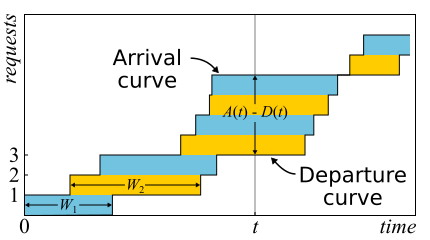 In mathematics it is often necessary to examine the evidence in order to get a real insight. This is the case. Little's theorem is so good that I give here a sketch of the proof. Incoming traffic is described by the function A ( t ) - the number of requests that have logged in to the point in time t . Similarly D ( t ) - the number of requests that left the system at the time t . The moment of entry (exit) of a request is considered the moment of receipt (transmission) of its last byte. The boundaries of the system are determined only by these points in time, so the theorem is obtained widely applicable. If you draw graphs of these functions in one axis, it is easy to see that A ( t ) - D ( t ) Is the number of requests in the system at time t, and W n - response time n-th request.
The theorem was formally proved only in 1961, although the relation itself was known long before that.
In fact, if requests within the system can be reordered, then everything is a bit more complicated, so for simplicity we will assume that this does not happen. Although the theorem is true in this case too. Now calculate the area between the graphs. This can be done in two ways. First, the columns - as is usually considered integrals. In this case, it turns out that the integrand is the size of the queue in pieces. Secondly, line by line - just by adding the latency of all requests. It is clear that both calculations give the same area, therefore they are equal. If both parts of this equality are divided by the time Δt for which we considered the area, then on the left we will have the average queue length L (by definition, average). The right is a little harder. It is necessary to insert in the numerator and denominator another number of queries N, then we will
It is important to say that in the proof we did not use any probability distributions. In fact, Little's theorem is a deterministic law! Such laws are called in the theory of queuing operational law. They can be applied to any parts of the system and any distributions of various random variables. These laws form a constructor that can be successfully used to analyze averages in networks. The disadvantage is that all of them are applicable only to average values and do not give any knowledge about distributions.
Returning to the question of why it is impossible to apply Little’s theorem to bytes, suppose A(t) and D(t) now measured not in pieces, but in bytes. Then, conducting a similar reasoning, we get instead W the weird thing is the area divided by the total number of bytes. This is still seconds, but it's something like weighted average latency, where larger requests get more weight. You can call this value the average latency of the byte - which is generally logical, since we replaced the pieces with bytes - but not the latency of the request.
Little's theorem says that with a certain flow of requests, the response time and the number of requests in the system are proportional. If all requests look the same, then the average response time cannot be reduced without increasing power. If we know the size of requests in advance, we can try to rearrange them internally to reduce the area between A(t) and D(t) and, therefore, the average response time of the system. Continuing this thought, one can prove that the Shortest Processing Time and Shortest Remaining Processing Time algorithms provide for a single server the minimum average response time without the possibility of crowding and with it, respectively. But there is a side effect - large requests can not be processed indefinitely. The phenomenon is called starvation and is closely related to the concept of fair planning, which can be found in the previous Scheduling post : myths and reality .
There is another common trap associated with understanding the law of Little. There is a single-threaded server that serves user requests. Suppose we somehow measured L - the average number of requests in the queue to this server, and S - the average service time for a single request by the server. Now consider the new incoming request. On average, he sees L requests ahead of him. The maintenance of each of them takes an average of S seconds. It turns out that the average waiting time W=LS . But by the theorem it turns out that W=L/ lambda . If we equate the expression, we see nonsense: S=1/ lambda . What is wrong with this reasoning?
So, Little's theorem can be applied to large and small systems, to queues, to servers and to single processing threads. But in all these cases, requests are usually classified in one way or another. Requests of different users, requests of different priority, requests coming from different locations, or requests of different types. In this case, the aggregated information by classes is not interesting. Yes, the average number of mixed requests and the average response time for all of them are proportional again. But what if we want to know the average response time for a particular class of requests? Surprisingly, Little's theorem can also be applied to a particular class of queries. In this case, you need to take as lambda rate of requests for this class, but not all. As L and W - average values of the number and residence time of requests of this class in the studied part of the system.
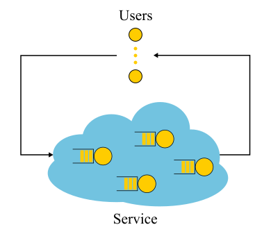 It should be noted that for closed systems the “wrong” line of reasoning leads to the conclusion S=1/ lambda turns out to be true. Closed systems are those systems in which requests do not come from the outside and do not go outside, but circulate inside. Or, alternatively, systems with feedback: as soon as a request leaves the system, a new request takes its place. These systems are also important because any open system can be viewed as immersed in a closed system. For example, you can consider the site as an open system, in which requests are constantly pouring in, processed and left, or you can, on the contrary, as a closed system with the entire audience of the site. Then they usually say that the number of users is fixed, and they either wait for the answer to the request, or “think”: they got their page and have not yet clicked on the link. In the event that the think time is always zero, the system is also called the batch system.
Little's law for closed systems is valid if the speed of external arrivals lambda (they are not in a closed system) replaced by the system bandwidth. If we wrap the single-threaded server, discussed above, into a batch system, we get S=1/ lambda and recycling 100%. Often such a look at the system gives unexpected results. In the 90s, it was this consideration of the Internet together with users as a unified system that gave impetus to the study of distributions other than exponential. We will discuss further distributions, but here we note that at that time almost everything and everywhere was regarded as exponential, and even found some justification for this, and not just an excuse in the spirit of "otherwise too complicated." However, it turned out that not all practically important distributions have equally long tails, and knowledge of distribution tails can be tried. But for now let us return to the average values.
Suppose we have an open system: a complex network or a simple single-threaded server is not important. What will change if we speed up the arrival of requests twice and speed up their processing twice - for example, having doubled the power of all the system components? How will the utilization, throughput, average number of requests in the system and the average response time change? For a single-threaded server, you can try to take the formulas, apply them "in the forehead" and get results, but what to do with an arbitrary network? Intuitive solution is as follows. Suppose that time has doubled in speed, then in our “accelerated reference system” the speed of the servers and the flow of requests did not seem to change; accordingly, all parameters in accelerated time have the same values as before. In other words, the acceleration of all the “moving parts” of any system is equivalent to the acceleration of a clock. Now convert the values to a system with normal time. The dimensionless quantities (utilization and average number of requests) will not change. Values whose dimension includes time multipliers of the first degree will change proportionally. The bandwidth [requests / s] will double, and the response and wait time [s] will be halved.
This result can be interpreted in two ways:
Once again, I note that this is true for a wide class of systems, and not just for a simple server. From a practical point of view, there are only two problems:
Consider the passage to the limit. Suppose, in the same open system, interpretation No. 2. We divide each incoming request in half. The response time is also divided in half. Repeat the division many times. And we do not even need to change anything in the system. It turns out that the response time can be made arbitrarily small by simply cutting incoming requests into a sufficiently large number of parts. In the limit, we can say that instead of requests, we get a “request fluid”, which we filter with our servers. This is the so-called fluid model, a very convenient tool for simplified analysis. But why is the response time zero? Something went wrong? In which place we did not take into account the latency? It turns out that we did not take into account the speed of light, it can not be doubled. The propagation time in the network channel cannot be changed; you can only accept it. In fact, transmission through a network includes two components: transmission time (propagation time) and propagation time (propagation time). The first can be accelerated by increasing the power (channel width) or reducing the size of the packets, and the second is very difficult to influence. In our “fluid model” there were just no reservoirs for the accumulation of liquids — network channels with non-zero and constant propagation time. By the way, if we add them to our “fluid model”, the latency will be determined by the sum of propagation times, and the queues at the nodes will still be empty. Queues depend only on the size of the packets and the variability (read burst) of the input stream.
From this it follows that if we are talking about latency, it is impossible to get by with the flow calculations, and even the disposal of devices does not solve everything. It is necessary to take into account the size of requests and not forget about the propagation time, which is often ignored in the queuing theory, although it is not at all difficult to add it to the calculations.
What is the general reason for the formation of queues? Obviously, there is not enough capacity in the system, and the excess of requests accumulates? Wrong! Queues also occur in systems where resources are sufficient. If the capacity is not enough, then the system, as the theorists say, is not stable. There are two main reasons for the formation of queues: the irregularity of the receipt of requests and the variability of the size of requests. We have already considered an example in which both of these reasons were eliminated: a real-time system, where requests of the same size come strictly periodically. The queue is never formed. The average waiting time in the queue is zero. It is clear that to achieve this behavior is very difficult, if not impossible, and therefore queues are formed. The queuing theory is based on the assumption that both causes are random and are described by some random variables.
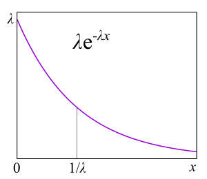
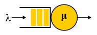 For the description of different systems used Kendall notation A / S / k / K, where A is the distribution of time between requests, S is the size distribution of requests, k is the number of servers, K is the limit on the simultaneous number of requests in the system (omitted if there is no limit). For example, the well-known M / M / 1 is deciphered as follows: the first M (Markovian or Memoryless) indicates that a Poisson flow of problems is fed to the system. Read: messages come at random times with a given average speed. lambda requests per second - just like radioactive decay - or, more formally: the time between two adjacent events has an exponential distribution. The second M indicates that the service of these messages also has an exponential distribution and, on average, μ requests are processed per second. Finally, a one at the end indicates that maintenance is performed by a single server. The queue is not limited, since the 4th part of the notation is absent. The letters used in this notation are rather strangely chosen: G is an arbitrary distribution (no, not Gaussian, as one might think), D is deterministic. Real-time system - D / D / 1. The first queuing theory system, which Erlang decided in 1909, is M / D / 1. But the analytic unresolved system so far is M / G / k for k> 1, and the solution for M / G / 1 was found back in 1930.
 The main reason is that they do almost any task about the queue being solved, because, as we will see, it becomes possible to apply Markov chains, about which mathematicians already know a lot of things. Exponential distributions have many good properties for a theory, because they do not have memory. I will not give here the definition of this property, for developers it will be more useful to explain through the failure rate . Suppose you have a certain device, but from practice you know the distribution of the lifetime of such devices: they often fail at the beginning of life, then break relatively rarely and after the warranty period expires, they often begin to break again. Formally, this information is precisely contained in the failure rate function, which is quite simply associated with the distribution. In fact, this is the “aligned” probability density given that the device has survived to a certain point. From a practical point of view, this is exactly what we are interested in: the frequency of device failures as a function of the time they are already in operation. For example, if the failure rate is a constant, that is, the failure rate of a device does not depend on the operation time, and failures just happen randomly at some frequency, then the distribution of the device lifetime is exponential. In this case, in order to predict how long the device will work, you do not need to know how long it has been in operation, what wear and tear it has and anything else. This is the "lack of memory."
Failure rate can be calculated for any distribution. In the theory of queuing - to distribute the time of the request. Failure rate , , , . failure rate, , , . failure rate, , , . , , , software hardware? : ? . , , - . ? , — . ( failure rate) . « » .
, , failure rate, , , unix- . , .
RTMR , . LWTrace - . . , . , P{S>x} . , failure rate , , : .
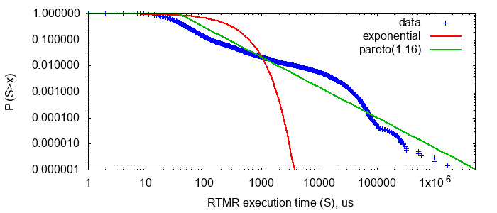
P{S>x}=x−a , — . , « », 80/20: , . . , . , RTMR -, , . Parameter a=1.16 , 80/20: 20% 80% .
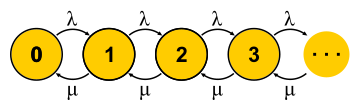 , . . , , , - . , — . « » , « » — . : , ? , ( , ), . , 0 . , , μN1 λN0 . , , — . . , . M/M/1 P{Q=i}=(1−ρ)ρi where ρ=λ/μ — . . , , , .
, , , , , . — . , , — failure rate.
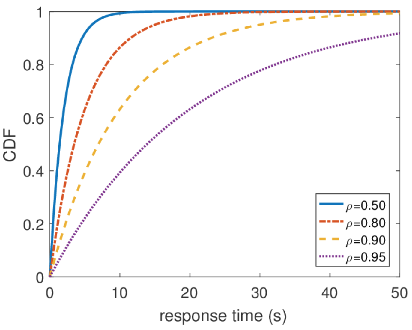 , , . — . , . , , P{response_time>t}=e−(μ−λ)t 1/(μ−λ) .
, , . , . , -, , . . , , , — . , , . , , . , , .
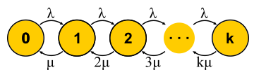 , , . . , . , . M/M/k/k M/M/k, . , . , , , , . M/M/k/k , , , , . , .
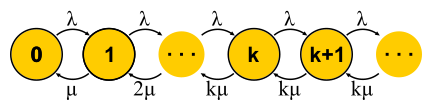 M/M/k , , , — . , M/M/1. , , , . . M/M/k/k M/M/k, B . , , , square root staffing rule. , M/M/k - λ . , . : , ? , ? , . , : ( ) , . — , . , M/M/1 , « » μ−λ . , , : 2μ−2λ . , , M/M/k . , « », . « » , : .
, , . , — M/M/k-. , , , — M/M/k, M/M/k , , . , , FIFO-. , , . , 10 , , . : .
, M/M/k, , . : . , , , . , M/M/k, . , , .
— . — . , , , , product-form solution . , — . . :
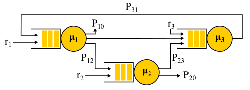 An example of the Jackson network.
It should be noted that in the presence of feedback the Poisson flow is NOT obtained, since the flows turn out to be interdependent. At the exit from the node with feedback, a non-Poisson flow is also obtained, and as a result, all flows become non-Poisson. However, surprisingly it turns out that all these non-Poisson flows behave exactly the same as the Poisson flows (oh, this probability theory), if the above limitations are fulfilled. And then we again get the product-form solution. Such networks are called Jackson networks , feedbacks are possible in them and, consequently, multiple visits to any server. There are other networks in which more liberties are allowed, but as a result all the significant analytical achievements of queuing theory in relation to networks imply Poisson flows at the entrance and a product-form solution, which became the subject of criticism of this theory and led in the 90s to the development of other theories, as well as to the study of what distributions are really needed and how to work with them.
An important application of this whole theory of Jackson networks is the modeling of packets in IP networks and ATM networks. The model is quite adequate: the packet sizes do not change much and do not depend on the packet itself, only on the channel width, since the service time corresponds to the packet transmission time to the channel. Random time of sending, although it sounds crazy, in fact, does not have very large variability. Moreover, it turns out that in a network with a deterministic service time, the latency cannot be greater than in a similar Jackson network, so such networks can be safely used to estimate the response time from above.
All the results that I talked about were exponential distributions, but I also mentioned that real distributions are different. There is a feeling that this whole theory is quite useless. This is not entirely true. There is a way to build in this mathematical apparatus and other distributions, moreover, almost any distributions, but it will cost us something. With the exception of a few interesting cases, the opportunity to get a solution is lost in an explicit form, the product-form solution is lost, and with it the constructor: each task must be solved entirely from scratch using Markov chains. For theory, this is a big problem, but in practice it simply means the use of numerical methods and makes it possible to solve much more complex and realistic problems.
The idea is simple. Markov chains do not allow us to have a memory inside one state, so all transitions must be random with an exponential time distribution between two transitions. But what if the state is divided into several substates? As before, transitions between substates must have an exponential distribution if we want the whole construction to remain a Markov chain, and we really want it, because we know how to solve such chains. Substates are often called phases, if they are arranged sequentially, and the partitioning process is called the phase method.
The simplest example. Processing the request is performed in several phases: first, for example, we read the necessary data from the database, then perform some calculations, then we write the results into the database. Suppose all these three stages have the same exponential distribution of time. What is the distribution time of passage of all three phases together? This is the Erlang distribution.
And what if you make many, many short identical phases? In the limit, we obtain a deterministic distribution. That is, building a chain, you can reduce the variability of the distribution.
Is it possible to increase the variability? Easy. Instead of a chain of phases, we use alternative categories, randomly choosing one of them. Example. Almost all requests are executed quickly, but there is a small chance that there will be a huge request that is executed for a long time. Such a distribution will have a decreasing failure rate. The longer we wait, the more likely it is that the request falls into the second category.

Continuing to develop the phase method, the theorists found out that there is a class of distributions, with the help of which one can approach with any accuracy an arbitrary nonnegative distribution! Coxian distibution is built using the phase method, only we do not have to go through all the phases, there is some probability of completion after each phase.
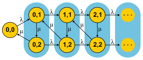
Such distributions can be used both to generate a non-Poisson input stream and to create a non-exponential service time. Here, for example, the Markov chain for the M / E2 / 1 system with Erlang distribution for service time. The state is determined by a pair of numbers (n, s), where n is the length of the queue, and s is the number of the stage in which the server is located: first or second. All combinations of n and s are possible. Incoming messages change only n, and upon completion of the phases they alternate and the queue length decreases after the completion of the second phase.
Can a system loaded at half its capacity slow down? As the first experimental, we dissect M / G / 1. Given: Poisson flow at the input and arbitrary distribution of service time. Consider the path of a single query through the entire system. Incoming incoming request sees the average number of requests in a queue in front of him mathbfE[NQ] . The average processing time of each of them mathbfE[S] . With probability equal to recycling rho , there is one more request in the server, which must first be “re-served” in time. mathbfE[Se] . Summing up, we get that the total waiting time in the queue mathbfE[TQ]= mathbfE[NQ] mathbfE[S]+ rho mathbfE[Se] . By Little's theorem mathbfE[NQ]= lambda mathbfE[TQ] ; combining, we get:

Average time mathbfE[Se] determined by the average value of the function Se(t) , that is, the area of the triangles divided by the total time. It is clear that we can confine ourselves to one "middle" triangle, then mathbfE[Se]= mathbfE[S2]/2 mathbfE[S] . This is quite unexpected. We have received that the time of after-service is determined not only by the average value of the service time, but also by its variation. The explanation is simple. The probability of falling into a long interval S more, it is actually proportional to the duration S of this interval. This explains the famous Waiting Time Paradox, or Inspection Paradox. But back to M / G / 1. If we combine everything that we have received and rewrite using the variability 2S= mathbfE[S]/ mathbfE[S]2 , we get the famous Pollaczek-Khinchine formula :
What do microbursts look like? In the case of trappools, these are tasks that are serviced fast enough so as not to be noticeable on the disposal schedules, and slowly enough to create a queue behind them and influence the response time of the pool. From the point of view of theory, these are huge requests from the tail part of the distribution. Let's say you have a pool of 10 threads, and you look at the recycling schedule, built on the metrics of work time and downtime, which are collected every 15 seconds. First, you may not notice that one thread generally hung, or that all 10 threads performed large tasks at the same time for a whole second, and then did nothing for 14 seconds. A resolution of 15 seconds does not allow to see a utilization jump of up to 100% and back to 0%, and the response time suffers. For example, this may look like microbirst, which happens every 15 seconds in a pool of 6 threads, if you look at it through a microscope.
As a microscope, a trace system is used that records the time of events (receipt and completion of requests) with an accuracy of processor cycles.
Especially in order to deal with such situations, RTMR uses the SelfPing mechanism, which periodically (every 10 ms) sends a small task to the trappool for the sole purpose of measuring the waiting time in the queue. Assuming the worst case, a period of 10 ms is added to this measurement and a maximum of 15 seconds is taken on the window. Thus, we get the upper estimate for the maximum waiting time on the window. Yes, we do not see the real state of affairs, if the response time is less than 10 ms, but in this case we can assume that everything is fine - there is not a single microbearst. But this additional self-ping activity eats a strictly limited amount of CPU. The mechanism is convenient in that it is universal and non-invasive: you do not need to change either the code of the trample or the code of the tasks that are executed in it. I emphasize: it is the worst case that is measured, which is very convenient and intuitive, compared to all sorts of percentiles. The mechanism also detects another similar situation: the simultaneous arrival of a large number of quite ordinary requests. If there are not so many of them, so that the problem could be seen on the 15-second disposal schedules, this can also be considered microbird.
Well, what if SelfPing shows that something is inadequate? How to find the guilty? To do this, we use the trace already mentioned LWTrace. We go to the problem machine and, through monitoring, we launch a trace, which keeps track of all the tasks in the right route and keeps only the slow ones in memory. Then you can see the top 100 slow runs. After a short study, turn off the trace. All other ways of searching for the guilty are not suitable: it is impossible to write logs for all the tasks of a trappool; writing only slow tasks is also not the best solution, since you still have to collect the track for all tasks, and this is also expensive; prof profiling with perf does not help, as hard tasks happen too rarely to be visible in a profile.
 We still have one more “degree of freedom”, which we have not used so far. We discussed the incoming flow and request sizes, different numbers of servers, too, but have not yet talked about schedulers. All examples implied FIFO processing. As I already mentioned, scheduling does affect the response time of the system, and the correct scheduler can significantly improve latency (SPT and SRPT algorithms). But planning is a very advanced topic for queuing theory. Perhaps this theory is not even very well suited for the study of planners, but this is the only theory that can provide answers to prochastic systems with schedulers and allows us to calculate averages. There are other theories that allow you to understand a lot about planning “at worst”, but we'll talk about them another time.
And now let's consider some interesting exceptions from the general rule, when you still manage to get a product-form solution for the network and you can create a convenient constructor. Let's start with one M / Cox / 1 / PS node. Poisson flow at the entrance, almost arbitrary distribution (Coxian distribution) of service time and fair scheduler (Processor Sharing), serving all requests at the same time, but with a speed inversely proportional to their current number. Where can I find such a system? For example, this is how fair process planners work in operating systems. At first glance it may seem that this is a complex system, but if you build (see the method section of the phases) and decide the corresponding Markov chain, it turns out that the distribution of the queue length exactly repeats the M / M / 1 / FIFO system , in which the service time has the same mean value, but is distributed exponentially.
This is an incredible result! In contrast to what we saw in the section on microbyls, here the variability of the maintenance time does not affect the response time in any of the percentiles! This property is rare and is called insensitivity property. Usually it occurs in systems where there is no waiting, and the request immediately starts to be executed in one way or another, when you do not need to wait until the after-care service of what is already being performed. Another example of a system with this property is M / M / ∞. It also has no expectations, as the number of servers is infinite. In such systems, the output stream from the node has a good distribution, which allows us to obtain a product-form solution for networks with such servers — BCMP networks .
 For completeness, consider the simplest example. Two servers operating at different average speeds (for example, the frequency of the processor is different), an arbitrary distribution of the sizes of incoming tasks, the service server is chosen randomly, most of the tasks go to the fast server. We need to find the average response time. Decision. mathbfE[T]=1/3 mathbfE[T1]+2/3 mathbfE[T2] . Apply the well-known formula mathbfE[Ti]=1/( mui− lambdai) for the average response time M / M / 1 / FCFS and get m a t h b f E [ T ] = 1 / 3 * 1 / ( 3 - 3 * 1 / 3 ) + 2 / 3 * 1 / ( 4 - 3 * 2 / 3 ) = 0.5 w i t h .
All right, now, and planning discussed, you can wrap up. In the next article, I will discuss how real-time systems approach the issue of latency and what concepts are used there.
My name is Sergey Trifonov, I work in the Real-Time Map Reduce team in Yandex. We are developing a real-time data streaming platform with seconds and sub-seconds response time. The platform is accessible to internal users and allows them to execute application code on constantly incoming data streams. I will try to make a brief overview of the basic concepts of humanity on the subject of latency analysis over the past hundred and ten years, and now we will try to understand what exactly latency can be learned by applying queuing theory.
The phenomenon of latency began to systematically explore, as far as I know, in connection with the emergence of queuing systems - telephone networks. The queuing theory began with the work of A. K. Erlang in 1909, in which he showed that the Poisson distribution is applicable to random telephone traffic. Erlang developed a theory that has been used for decades to design telephone networks. The theory allows you to determine the probability of failure in service. For circuit-switched telephone networks, a failure occurred if all channels were busy and the call could not be completed. The probability of this event had to be controlled. I wanted to have a guarantee that, for example, 95% of all calls will be served. Erlang's formulas allow you to determine how many servers are needed to fulfill this guarantee, if the duration and number of calls is known. In fact, this task is about quality assurance, and today people are still solving similar problems. But systems have become much more complicated. The main problem of the queuing theory is that in most institutions it is not taught, and few people understand the question beyond the usual M / M / 1 queue (see about the notation below ), but it is well known that life is much more complicated than this system. Therefore, I suggest, bypassing M / M / 1, go directly to the most interesting.
Average values
If you do not try to gain complete knowledge of the probability distribution in the system, and focus on simpler questions, you can get interesting and useful results. The most famous of them is, of course, the Little theorem . It is applicable to a system with any input stream, internal device of any complexity and an arbitrary scheduler inside. The only requirement is that the system must be stable: there must be average values of response time and queue length, then they are connected by a simple expression
L = l a m b d a W
where L - time average number of requests in the considered part of the system [piece], W - the average time for which requests pass through this part of the system [s], l a m b d a - the rate of requests in the system [pcs / s]. The strength of the theorem is that it can be applied to any part of the system: the queue, the performer, the queue + the performer, or the entire network. Often this theorem is used approximately like this: “The stream of 1Gbit / s flows to us, and we measured the average response time, and it is 10 ms, so we have an average of 1.25 MB in flight”. So, this calculation is not true. More precisely, it is true, only if all requests have the same size in bytes. Little's theorem counts requests in pieces, not in bytes.
')
How to use Little's theorem
In mathematics it is often necessary to examine the evidence in order to get a real insight. This is the case. Little's theorem is so good that I give here a sketch of the proof. Incoming traffic is described by the function A ( t ) - the number of requests that have logged in to the point in time t . Similarly D ( t ) - the number of requests that left the system at the time t . The moment of entry (exit) of a request is considered the moment of receipt (transmission) of its last byte. The boundaries of the system are determined only by these points in time, so the theorem is obtained widely applicable. If you draw graphs of these functions in one axis, it is easy to see that A ( t ) - D ( t ) Is the number of requests in the system at time t, and W n - response time n-th request.The theorem was formally proved only in 1961, although the relation itself was known long before that.
In fact, if requests within the system can be reordered, then everything is a bit more complicated, so for simplicity we will assume that this does not happen. Although the theorem is true in this case too. Now calculate the area between the graphs. This can be done in two ways. First, the columns - as is usually considered integrals. In this case, it turns out that the integrand is the size of the queue in pieces. Secondly, line by line - just by adding the latency of all requests. It is clear that both calculations give the same area, therefore they are equal. If both parts of this equality are divided by the time Δt for which we considered the area, then on the left we will have the average queue length L (by definition, average). The right is a little harder. It is necessary to insert in the numerator and denominator another number of queries N, then we will
frac sumWi Deltat= frac sumWiN fracN Deltat=W lambda
If we consider sufficiently large Δt or one period of employment, then questions on the edges are removed and the theorem can be considered proven.
It is important to say that in the proof we did not use any probability distributions. In fact, Little's theorem is a deterministic law! Such laws are called in the theory of queuing operational law. They can be applied to any parts of the system and any distributions of various random variables. These laws form a constructor that can be successfully used to analyze averages in networks. The disadvantage is that all of them are applicable only to average values and do not give any knowledge about distributions.
Returning to the question of why it is impossible to apply Little’s theorem to bytes, suppose A(t) and D(t) now measured not in pieces, but in bytes. Then, conducting a similar reasoning, we get instead W the weird thing is the area divided by the total number of bytes. This is still seconds, but it's something like weighted average latency, where larger requests get more weight. You can call this value the average latency of the byte - which is generally logical, since we replaced the pieces with bytes - but not the latency of the request.
Little's theorem says that with a certain flow of requests, the response time and the number of requests in the system are proportional. If all requests look the same, then the average response time cannot be reduced without increasing power. If we know the size of requests in advance, we can try to rearrange them internally to reduce the area between A(t) and D(t) and, therefore, the average response time of the system. Continuing this thought, one can prove that the Shortest Processing Time and Shortest Remaining Processing Time algorithms provide for a single server the minimum average response time without the possibility of crowding and with it, respectively. But there is a side effect - large requests can not be processed indefinitely. The phenomenon is called starvation and is closely related to the concept of fair planning, which can be found in the previous Scheduling post : myths and reality .
There is another common trap associated with understanding the law of Little. There is a single-threaded server that serves user requests. Suppose we somehow measured L - the average number of requests in the queue to this server, and S - the average service time for a single request by the server. Now consider the new incoming request. On average, he sees L requests ahead of him. The maintenance of each of them takes an average of S seconds. It turns out that the average waiting time W=LS . But by the theorem it turns out that W=L/ lambda . If we equate the expression, we see nonsense: S=1/ lambda . What is wrong with this reasoning?
- The first thing that catches the eye: the response time by the theorem does not depend on S. In fact, of course, it depends. Simply, the average queue length already takes this into account: the faster the server, the shorter the queue length and the shorter the response time.
- We consider a system in which the queues do not accumulate forever, but are regularly reset. This means that server utilization is less than 100% and we skip all incoming requests, and with the same average speed with which these requests came, which means, on average, processing one request takes not S seconds, but more 1/ lambda seconds, simply because sometimes we do not process any requests. The fact is that in any stable open system without loss the throughput does not depend on the speed of the servers, it is determined only by the input stream.
- The assumption that an incoming request sees the average number of requests in the system is not always true. A counterexample: incoming requests come strictly periodically, and we manage to process each request before the next one arrives. Typical picture for real-time systems. An incoming request always sees a zero in the system, but on average in the system, obviously, more than zero requests. If requests come at completely random times, then they really "see the average number of requests . "
- We did not take into account that with some probability there can already be one request in the server that needs to be “re-served”. In general, the average “after-service” time differs from the initial service time, and sometimes, paradoxically , it can be much longer. We will return to this question at the end, when we discuss microbursts, stay tuned.
So, Little's theorem can be applied to large and small systems, to queues, to servers and to single processing threads. But in all these cases, requests are usually classified in one way or another. Requests of different users, requests of different priority, requests coming from different locations, or requests of different types. In this case, the aggregated information by classes is not interesting. Yes, the average number of mixed requests and the average response time for all of them are proportional again. But what if we want to know the average response time for a particular class of requests? Surprisingly, Little's theorem can also be applied to a particular class of queries. In this case, you need to take as lambda rate of requests for this class, but not all. As L and W - average values of the number and residence time of requests of this class in the studied part of the system.
Open and closed systems
It should be noted that for closed systems the “wrong” line of reasoning leads to the conclusion S=1/ lambda turns out to be true. Closed systems are those systems in which requests do not come from the outside and do not go outside, but circulate inside. Or, alternatively, systems with feedback: as soon as a request leaves the system, a new request takes its place. These systems are also important because any open system can be viewed as immersed in a closed system. For example, you can consider the site as an open system, in which requests are constantly pouring in, processed and left, or you can, on the contrary, as a closed system with the entire audience of the site. Then they usually say that the number of users is fixed, and they either wait for the answer to the request, or “think”: they got their page and have not yet clicked on the link. In the event that the think time is always zero, the system is also called the batch system.Little's law for closed systems is valid if the speed of external arrivals lambda (they are not in a closed system) replaced by the system bandwidth. If we wrap the single-threaded server, discussed above, into a batch system, we get S=1/ lambda and recycling 100%. Often such a look at the system gives unexpected results. In the 90s, it was this consideration of the Internet together with users as a unified system that gave impetus to the study of distributions other than exponential. We will discuss further distributions, but here we note that at that time almost everything and everywhere was regarded as exponential, and even found some justification for this, and not just an excuse in the spirit of "otherwise too complicated." However, it turned out that not all practically important distributions have equally long tails, and knowledge of distribution tails can be tried. But for now let us return to the average values.
Relativistic effects
Suppose we have an open system: a complex network or a simple single-threaded server is not important. What will change if we speed up the arrival of requests twice and speed up their processing twice - for example, having doubled the power of all the system components? How will the utilization, throughput, average number of requests in the system and the average response time change? For a single-threaded server, you can try to take the formulas, apply them "in the forehead" and get results, but what to do with an arbitrary network? Intuitive solution is as follows. Suppose that time has doubled in speed, then in our “accelerated reference system” the speed of the servers and the flow of requests did not seem to change; accordingly, all parameters in accelerated time have the same values as before. In other words, the acceleration of all the “moving parts” of any system is equivalent to the acceleration of a clock. Now convert the values to a system with normal time. The dimensionless quantities (utilization and average number of requests) will not change. Values whose dimension includes time multipliers of the first degree will change proportionally. The bandwidth [requests / s] will double, and the response and wait time [s] will be halved.
This result can be interpreted in two ways:
- Accelerated k times the system can digest the flow of tasks k times more, and with an average response time k times less.
- We can say that the power has not changed, but simply the size of the tasks has decreased by k times. It turns out that we are sending the same load into the system, but sawn into smaller pieces. And ... lo and behold! Average response time decreases!
Once again, I note that this is true for a wide class of systems, and not just for a simple server. From a practical point of view, there are only two problems:
- Not all parts of the system can be easily accelerated. For some, we can not affect in any way at all. For example, at the speed of light.
- Not all tasks can be infinitely divided into smaller ones, since they have not learned to transmit information in portions of less than one bit.
Consider the passage to the limit. Suppose, in the same open system, interpretation No. 2. We divide each incoming request in half. The response time is also divided in half. Repeat the division many times. And we do not even need to change anything in the system. It turns out that the response time can be made arbitrarily small by simply cutting incoming requests into a sufficiently large number of parts. In the limit, we can say that instead of requests, we get a “request fluid”, which we filter with our servers. This is the so-called fluid model, a very convenient tool for simplified analysis. But why is the response time zero? Something went wrong? In which place we did not take into account the latency? It turns out that we did not take into account the speed of light, it can not be doubled. The propagation time in the network channel cannot be changed; you can only accept it. In fact, transmission through a network includes two components: transmission time (propagation time) and propagation time (propagation time). The first can be accelerated by increasing the power (channel width) or reducing the size of the packets, and the second is very difficult to influence. In our “fluid model” there were just no reservoirs for the accumulation of liquids — network channels with non-zero and constant propagation time. By the way, if we add them to our “fluid model”, the latency will be determined by the sum of propagation times, and the queues at the nodes will still be empty. Queues depend only on the size of the packets and the variability (read burst) of the input stream.
From this it follows that if we are talking about latency, it is impossible to get by with the flow calculations, and even the disposal of devices does not solve everything. It is necessary to take into account the size of requests and not forget about the propagation time, which is often ignored in the queuing theory, although it is not at all difficult to add it to the calculations.
Distributions
What is the general reason for the formation of queues? Obviously, there is not enough capacity in the system, and the excess of requests accumulates? Wrong! Queues also occur in systems where resources are sufficient. If the capacity is not enough, then the system, as the theorists say, is not stable. There are two main reasons for the formation of queues: the irregularity of the receipt of requests and the variability of the size of requests. We have already considered an example in which both of these reasons were eliminated: a real-time system, where requests of the same size come strictly periodically. The queue is never formed. The average waiting time in the queue is zero. It is clear that to achieve this behavior is very difficult, if not impossible, and therefore queues are formed. The queuing theory is based on the assumption that both causes are random and are described by some random variables.
For the description of different systems used Kendall notation A / S / k / K, where A is the distribution of time between requests, S is the size distribution of requests, k is the number of servers, K is the limit on the simultaneous number of requests in the system (omitted if there is no limit). For example, the well-known M / M / 1 is deciphered as follows: the first M (Markovian or Memoryless) indicates that a Poisson flow of problems is fed to the system. Read: messages come at random times with a given average speed. lambda requests per second - just like radioactive decay - or, more formally: the time between two adjacent events has an exponential distribution. The second M indicates that the service of these messages also has an exponential distribution and, on average, μ requests are processed per second. Finally, a one at the end indicates that maintenance is performed by a single server. The queue is not limited, since the 4th part of the notation is absent. The letters used in this notation are rather strangely chosen: G is an arbitrary distribution (no, not Gaussian, as one might think), D is deterministic. Real-time system - D / D / 1. The first queuing theory system, which Erlang decided in 1909, is M / D / 1. But the analytic unresolved system so far is M / G / k for k> 1, and the solution for M / G / 1 was found back in 1930.Why use exponential distributions?
The main reason is that they do almost any task about the queue being solved, because, as we will see, it becomes possible to apply Markov chains, about which mathematicians already know a lot of things. Exponential distributions have many good properties for a theory, because they do not have memory. I will not give here the definition of this property, for developers it will be more useful to explain through the failure rate . Suppose you have a certain device, but from practice you know the distribution of the lifetime of such devices: they often fail at the beginning of life, then break relatively rarely and after the warranty period expires, they often begin to break again. Formally, this information is precisely contained in the failure rate function, which is quite simply associated with the distribution. In fact, this is the “aligned” probability density given that the device has survived to a certain point. From a practical point of view, this is exactly what we are interested in: the frequency of device failures as a function of the time they are already in operation. For example, if the failure rate is a constant, that is, the failure rate of a device does not depend on the operation time, and failures just happen randomly at some frequency, then the distribution of the device lifetime is exponential. In this case, in order to predict how long the device will work, you do not need to know how long it has been in operation, what wear and tear it has and anything else. This is the "lack of memory."Short and long tails
Failure rate can be calculated for any distribution. In the theory of queuing - to distribute the time of the request. Failure rate , , , . failure rate, , , . failure rate, , , . , , , software hardware? : ? . , , - . ? , — . ( failure rate) . « » .
, , failure rate, , , unix- . , .
RTMR , . LWTrace - . . , . , P{S>x} . , failure rate , , : .
P{S>x}=x−a , — . , « », 80/20: , . . , . , RTMR -, , . Parameter a=1.16 , 80/20: 20% 80% .
, . . , , , - . , — . « » , « » — . : , ? , ( , ), . , 0 . , , μN1 λN0 . , , — . . , . M/M/1 P{Q=i}=(1−ρ)ρi where ρ=λ/μ — . . , , , ., , , , , . — . , , — failure rate.
, , . — . , . , , P{response_time>t}=e−(μ−λ)t 1/(μ−λ) ., , . , . , -, , . . , , , — . , , . , , . , , .
, , . . , . , . M/M/k/k M/M/k, . , . , , , , . M/M/k/k , , , , . , . M/M/k , , , — . , M/M/1. , , , . . M/M/k/k M/M/k, B . , , , square root staffing rule. , M/M/k - λ . , . : , ? , ? , . , : ( ) , . — , . , M/M/1 , « » μ−λ . , , : 2μ−2λ . , , M/M/k . , « », . « » , : ., , . , — M/M/k-. , , , — M/M/k, M/M/k , , . , , FIFO-. , , . , 10 , , . : .
, M/M/k, , . : . , , , . , M/M/k, . , , .
— . — . , , , , product-form solution . , — . . :
- . , , . , , « »: , № 1, № 2 , № 2, № 1 № 3 . , 100%- .
- . , , . , , . . — . , , , , .
- .
It should be noted that in the presence of feedback the Poisson flow is NOT obtained, since the flows turn out to be interdependent. At the exit from the node with feedback, a non-Poisson flow is also obtained, and as a result, all flows become non-Poisson. However, surprisingly it turns out that all these non-Poisson flows behave exactly the same as the Poisson flows (oh, this probability theory), if the above limitations are fulfilled. And then we again get the product-form solution. Such networks are called Jackson networks , feedbacks are possible in them and, consequently, multiple visits to any server. There are other networks in which more liberties are allowed, but as a result all the significant analytical achievements of queuing theory in relation to networks imply Poisson flows at the entrance and a product-form solution, which became the subject of criticism of this theory and led in the 90s to the development of other theories, as well as to the study of what distributions are really needed and how to work with them.
An important application of this whole theory of Jackson networks is the modeling of packets in IP networks and ATM networks. The model is quite adequate: the packet sizes do not change much and do not depend on the packet itself, only on the channel width, since the service time corresponds to the packet transmission time to the channel. Random time of sending, although it sounds crazy, in fact, does not have very large variability. Moreover, it turns out that in a network with a deterministic service time, the latency cannot be greater than in a similar Jackson network, so such networks can be safely used to estimate the response time from above.
Nonexponential distributions
All the results that I talked about were exponential distributions, but I also mentioned that real distributions are different. There is a feeling that this whole theory is quite useless. This is not entirely true. There is a way to build in this mathematical apparatus and other distributions, moreover, almost any distributions, but it will cost us something. With the exception of a few interesting cases, the opportunity to get a solution is lost in an explicit form, the product-form solution is lost, and with it the constructor: each task must be solved entirely from scratch using Markov chains. For theory, this is a big problem, but in practice it simply means the use of numerical methods and makes it possible to solve much more complex and realistic problems.
Phase method
The idea is simple. Markov chains do not allow us to have a memory inside one state, so all transitions must be random with an exponential time distribution between two transitions. But what if the state is divided into several substates? As before, transitions between substates must have an exponential distribution if we want the whole construction to remain a Markov chain, and we really want it, because we know how to solve such chains. Substates are often called phases, if they are arranged sequentially, and the partitioning process is called the phase method.
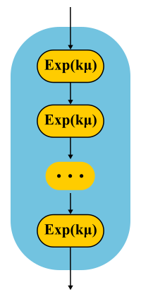
The simplest example. Processing the request is performed in several phases: first, for example, we read the necessary data from the database, then perform some calculations, then we write the results into the database. Suppose all these three stages have the same exponential distribution of time. What is the distribution time of passage of all three phases together? This is the Erlang distribution.
And what if you make many, many short identical phases? In the limit, we obtain a deterministic distribution. That is, building a chain, you can reduce the variability of the distribution.
Is it possible to increase the variability? Easy. Instead of a chain of phases, we use alternative categories, randomly choosing one of them. Example. Almost all requests are executed quickly, but there is a small chance that there will be a huge request that is executed for a long time. Such a distribution will have a decreasing failure rate. The longer we wait, the more likely it is that the request falls into the second category.
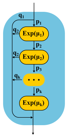
Continuing to develop the phase method, the theorists found out that there is a class of distributions, with the help of which one can approach with any accuracy an arbitrary nonnegative distribution! Coxian distibution is built using the phase method, only we do not have to go through all the phases, there is some probability of completion after each phase.
Such distributions can be used both to generate a non-Poisson input stream and to create a non-exponential service time. Here, for example, the Markov chain for the M / E2 / 1 system with Erlang distribution for service time. The state is determined by a pair of numbers (n, s), where n is the length of the queue, and s is the number of the stage in which the server is located: first or second. All combinations of n and s are possible. Incoming messages change only n, and upon completion of the phases they alternate and the queue length decreases after the completion of the second phase.
You have mikrobersty!
Can a system loaded at half its capacity slow down? As the first experimental, we dissect M / G / 1. Given: Poisson flow at the input and arbitrary distribution of service time. Consider the path of a single query through the entire system. Incoming incoming request sees the average number of requests in a queue in front of him mathbfE[NQ] . The average processing time of each of them mathbfE[S] . With probability equal to recycling rho , there is one more request in the server, which must first be “re-served” in time. mathbfE[Se] . Summing up, we get that the total waiting time in the queue mathbfE[TQ]= mathbfE[NQ] mathbfE[S]+ rho mathbfE[Se] . By Little's theorem mathbfE[NQ]= lambda mathbfE[TQ] ; combining, we get:
mathbfE[TQ]= frac rho1− rho mathbfE[Se]
That is, the waiting time in the queue is determined by two factors. The first is the effect of server recycling, and the second is the average after-service time. Consider the second factor. Request coming at some point t , sees that it takes time to pre-service Se(t) .
Average time mathbfE[Se] determined by the average value of the function Se(t) , that is, the area of the triangles divided by the total time. It is clear that we can confine ourselves to one "middle" triangle, then mathbfE[Se]= mathbfE[S2]/2 mathbfE[S] . This is quite unexpected. We have received that the time of after-service is determined not only by the average value of the service time, but also by its variation. The explanation is simple. The probability of falling into a long interval S more, it is actually proportional to the duration S of this interval. This explains the famous Waiting Time Paradox, or Inspection Paradox. But back to M / G / 1. If we combine everything that we have received and rewrite using the variability 2S= mathbfE[S]/ mathbfE[S]2 , we get the famous Pollaczek-Khinchine formula :
mathbfE[TQ]= frac rho1− rho frac mathbfE[S]2(C2S+1)
If the proof is tired of you, I hope, the result of practical application will please you. We have already studied the service time data in RTMR. A long tail just occurs with great variability and in this case C2S=$38 . This, you will agree, is much more than C2S=1 for exponential distribution. On average, everything is super fast: m a t h b f E [ S ] = 263.792 μ s . Now suppose that RTMR is modeled by the M / G / 1 system, and let the system not be heavily loaded, the recycling rho=0.5 . Substituting in the formula, we get mathbfE[TQ]=1∗(381+1)/2∗263.792μs=50ms . Because of microbursts, even such a fast and under-utilized system can, on average, become disgusting. For 50 ms, you can go to the hard drive 6 times or, if you're lucky, even to a data center on another continent! By the way, for G / G / 1 there is an approximation that takes into account the variability of incoming traffic: it looks exactly the same, only instead C2S+1 in it the sum of both variations C2S+C2A . For a case with several servers, things are better, but the effect of several servers only affects the first multiplier. The effect of variability remains: mathbfE[TQ]G/G/k≈ mathbfE[TQ]M/M/k(C2S+C2A)/2 .
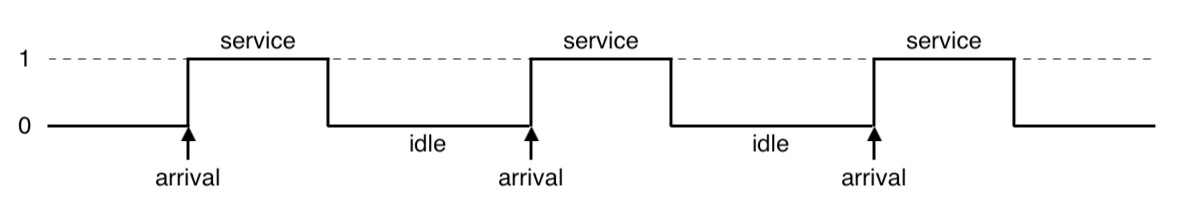
What do microbursts look like? In the case of trappools, these are tasks that are serviced fast enough so as not to be noticeable on the disposal schedules, and slowly enough to create a queue behind them and influence the response time of the pool. From the point of view of theory, these are huge requests from the tail part of the distribution. Let's say you have a pool of 10 threads, and you look at the recycling schedule, built on the metrics of work time and downtime, which are collected every 15 seconds. First, you may not notice that one thread generally hung, or that all 10 threads performed large tasks at the same time for a whole second, and then did nothing for 14 seconds. A resolution of 15 seconds does not allow to see a utilization jump of up to 100% and back to 0%, and the response time suffers. For example, this may look like microbirst, which happens every 15 seconds in a pool of 6 threads, if you look at it through a microscope.
As a microscope, a trace system is used that records the time of events (receipt and completion of requests) with an accuracy of processor cycles.
Especially in order to deal with such situations, RTMR uses the SelfPing mechanism, which periodically (every 10 ms) sends a small task to the trappool for the sole purpose of measuring the waiting time in the queue. Assuming the worst case, a period of 10 ms is added to this measurement and a maximum of 15 seconds is taken on the window. Thus, we get the upper estimate for the maximum waiting time on the window. Yes, we do not see the real state of affairs, if the response time is less than 10 ms, but in this case we can assume that everything is fine - there is not a single microbearst. But this additional self-ping activity eats a strictly limited amount of CPU. The mechanism is convenient in that it is universal and non-invasive: you do not need to change either the code of the trample or the code of the tasks that are executed in it. I emphasize: it is the worst case that is measured, which is very convenient and intuitive, compared to all sorts of percentiles. The mechanism also detects another similar situation: the simultaneous arrival of a large number of quite ordinary requests. If there are not so many of them, so that the problem could be seen on the 15-second disposal schedules, this can also be considered microbird.
Well, what if SelfPing shows that something is inadequate? How to find the guilty? To do this, we use the trace already mentioned LWTrace. We go to the problem machine and, through monitoring, we launch a trace, which keeps track of all the tasks in the right route and keeps only the slow ones in memory. Then you can see the top 100 slow runs. After a short study, turn off the trace. All other ways of searching for the guilty are not suitable: it is impossible to write logs for all the tasks of a trappool; writing only slow tasks is also not the best solution, since you still have to collect the track for all tasks, and this is also expensive; prof profiling with perf does not help, as hard tasks happen too rarely to be visible in a profile.
Independence from service time allocation
We still have one more “degree of freedom”, which we have not used so far. We discussed the incoming flow and request sizes, different numbers of servers, too, but have not yet talked about schedulers. All examples implied FIFO processing. As I already mentioned, scheduling does affect the response time of the system, and the correct scheduler can significantly improve latency (SPT and SRPT algorithms). But planning is a very advanced topic for queuing theory. Perhaps this theory is not even very well suited for the study of planners, but this is the only theory that can provide answers to prochastic systems with schedulers and allows us to calculate averages. There are other theories that allow you to understand a lot about planning “at worst”, but we'll talk about them another time.And now let's consider some interesting exceptions from the general rule, when you still manage to get a product-form solution for the network and you can create a convenient constructor. Let's start with one M / Cox / 1 / PS node. Poisson flow at the entrance, almost arbitrary distribution (Coxian distribution) of service time and fair scheduler (Processor Sharing), serving all requests at the same time, but with a speed inversely proportional to their current number. Where can I find such a system? For example, this is how fair process planners work in operating systems. At first glance it may seem that this is a complex system, but if you build (see the method section of the phases) and decide the corresponding Markov chain, it turns out that the distribution of the queue length exactly repeats the M / M / 1 / FIFO system , in which the service time has the same mean value, but is distributed exponentially.
This is an incredible result! In contrast to what we saw in the section on microbyls, here the variability of the maintenance time does not affect the response time in any of the percentiles! This property is rare and is called insensitivity property. Usually it occurs in systems where there is no waiting, and the request immediately starts to be executed in one way or another, when you do not need to wait until the after-care service of what is already being performed. Another example of a system with this property is M / M / ∞. It also has no expectations, as the number of servers is infinite. In such systems, the output stream from the node has a good distribution, which allows us to obtain a product-form solution for networks with such servers — BCMP networks .
For completeness, consider the simplest example. Two servers operating at different average speeds (for example, the frequency of the processor is different), an arbitrary distribution of the sizes of incoming tasks, the service server is chosen randomly, most of the tasks go to the fast server. We need to find the average response time. Decision. mathbfE[T]=1/3 mathbfE[T1]+2/3 mathbfE[T2] . Apply the well-known formula mathbfE[Ti]=1/( mui− lambdai) for the average response time M / M / 1 / FCFS and get m a t h b f E [ T ] = 1 / 3 * 1 / ( 3 - 3 * 1 / 3 ) + 2 / 3 * 1 / ( 4 - 3 * 2 / 3 ) = 0.5 w i t h .All right, now, and planning discussed, you can wrap up. In the next article, I will discuss how real-time systems approach the issue of latency and what concepts are used there.
What to read and see
- The study of queuing theory is always accompanied by a rather keen mathematics, and often the systems that are considered have nothing to do with computer science, so it’s hard to find a good tutorial. I would recommend Performance Modeling and Design of Computer Systems (2013). There is still enough mathematics, but all of it is attached to interesting systems. Most of this article is a free retelling of this book.
- The simplest, to the extent possible, without loss of meaning, is the presentation of the classics of the theory about which I know, in the format of video lectures of Robert B. Cooper. In these lectures, he very lucidly tells almost his entire book and everything that is required for its understanding.
Source: https://habr.com/ru/post/431650/
All Articles