Julia. Strings and Metaprogramming

We continue to study the young and promising general-purpose language Julia . At this time, we will pay more attention to the lines, begin timid steps into the world of metaprogramming and teach the interpreter to perform symbolic operations (There are only two pictures under the cut, but a lot of syntactic sugar)

Strings

String variables are created using a frame of characters in double quotes, and single characters of type char are entered as single characters. String concatenation is performed using multiplication "*":

cats = 4 s1 = "How many cats "; s2 = "is too many cats?"; s3 = s1*s2 Out[]: "How many cats is too many cats?" 

That is, the exponentiation works like this:

 s1^3 Out[]: "How many cats How many cats How many cats " 

On the other hand, indexing is extended to lines:

 s1[3] Out[]: 'w': ASCII/Unicode U+0077 (category Ll: Letter, lowercase) s1[5:13] Out[]: "many cats" s1[13:-1:5] Out[]: "stac ynam" s2[end] Out[]: '?': ASCII/Unicode U+003f (category Po: Punctuation, other) 

Strings can be created from strings and other types:

 s4 = string(s3, " - I don't know, but ", cats, " is too few.") #   s4 = "$s3 - I don't know, but $cats is too few." Out[]: "How many cats is too many cats? - I don't know, but 4 is too few." 

There are many useful functions in the arsenal, for example, the search for an element:

 findfirst( isequal('o'), s4 ) Out[]: 4 findlast( isequal('o'), s4 ) Out[]: 26 findnext( isequal('o'), s4, 7 ) #      Out[]: 11 

And this is how you can easily implement Caesar's Cipher

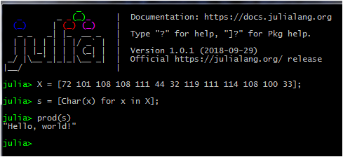
 caesar(X, n) = prod( [x += n for x in X] ) str3 = "    "; caesar(str3, 3) Out[]: "####" str4 = caesar(str3, -32) Out[]: "\0\0\0\0" "Latin letters go before Cyrillic" < str4 < str3 Out[]: true 

Here there is a run through all the characters of the string, to the code of each of which is added n . It turns out an array of char characters, which are glued together by the prod () function, which implements the multiplication of all elements of the received array.

Character calculations

Julia for symbolic calculations already has packages of different degrees of readiness, for example:

• Sympy
• Symata
• SymEngine
• LinearExpressions

but we learned how to glue strings together, why not implement symbolic actions with matrices. Let's say we wanted to add two bitty arrays:

 m1 = [1 1 "a"; 1 0 1] Out[]: 2×3 Array{Any,2}: 1 1 "a" 1 0 1 m3 = [1 2 "ln(3)"; 2 1 0] Out[]: 2×3 Array{Any,2}: 1 2 "ln(3)" 2 1 0 m1+m3 Out[]: MethodError: no method matching +(::String, ::String) ... 

To begin with, let's launch our playful hands to the basic operators:

 import Base: *, -, + 

If in C ++, such a mulling was called operator overloading, here we simply add a method for an existing function.

 +(a::String, b::String) = a * "+" * b Out[]: + (generic function with 164 methods) 

More than a hundred and fifty methods, and here's another one that will live until the end of the session.

 m1+m3 Out[]: 2×3 Array{Any,2}: 2 3 "a+ln(3)" 3 1 1 

Now we subtract multiplication, namely, we define the case of multiplying a string by a number:

 function *(a::String, b::Number) if b == 0 0 else if b == 1 a else "$b" * "*(" * a * ")" end end end Out[]: * (generic function with 344 methods) 

That is, if the string is multiplied by zero, we get zero, if by one, we get the string itself, and in other cases, we merge the number with the “*” sign and with the string (the brackets added so that there are no ambiguities with signs). Personally, I like the single-line view of the function, for which the ternary operator is useful:

 *(a::String, b::Number) = (b==0) ? 0 : (b==1) ? a : "$b" * "*(" * a * ")" Out[]: 

Expose the rest of cases to similar executions and get something like:

 import Base: *, -, + +(a::String, b::String) = a * "+" * b *(a::String, b::String) = a * "*(" * b * ")" *(a::String, b::Number) = (b==0) ? 0 : (b==1) ? a : "$b" * "*(" * a * ")" *(b::Number, a::String) = (b==0) ? 0 : (b==1) ? a : "$b" * "*(" * a * ")" +(a::String, b::Number) = (b==0) ? a : a * "+" * "$b" +(b::Number, a::String) = (b==0) ? a : a * "+" * "$b" -(b::Number, a::String) = (b==0) ? "-" * a : "$b" * "-" * a -(a::String, b::Number) = (b==0) ? a : a * "-" * "$b" # m1 = [1 1 "a"; 1 0 1] m2 = [2 0 2; 2 "b" 2; 2 2 2] m1*m2 Out[]: 2×3 Array{Any,2}: "2*(a)+4" "b+2*(a)" "2*(a)+4" 4 2 4 

And let's calculate the determinant! But since the built-in function is difficult, our methods are not enough to feed the matrix with strings to it - we get an error. So we are quick to implement our own using the Levi-Civita symbol

 ε = zeros(Int, 3,3,3) ε[1,2,3] = ε[2,3,1] = ε[3,1,2] = 1 ε[3,2,1] = ε[1,3,2] = ε[2,1,3] = -1 ε Out[]: 3×3×3 Array{Int64,3}: [:, :, 1] = 0 0 0 0 0 1 0 -1 0 [:, :, 2] = 0 0 -1 0 0 0 1 0 0 [:, :, 3] = 0 1 0 -1 0 0 0 0 0 

Mixed Formula

$$

$$\ left [\ vec {a} \ vec {b} \ vec {c} \ right] = \ sum_ {i, j, k = 1} ^ {3} \ varepsilon_ {ijk} a ^ ib ^ jc ^ k$$

can be used to find the determinant of a 3x3 matrix, understanding a , b , c as the first, second and third row (column), respectively

 detrmnt(arr) = sum( ε[i,j,k]*arr[1,i]*arr[2,j]*arr[3,k] for i in 1:3, j in 1:3, k in 1:3 ) detrmnt(["a" 2 "b"; 1 0 1; "c" 2 "d"]) Out[]: "2*(c)+2*(b)+2*(-1*(a))+-2*(d)" 

It is not difficult to guess that it is more difficult for matrices, everything will look very nontrivial - a set of brackets and multiplications of numbers, so it would be nice to make a couple of functions conducting defactorization. This will be your homework.
In addition, multiplication of arrays is more complicated:

 Rx = [1 0 0 0; 0 "cos(ϕ)" "sin(ϕ)" 0; 0 "-sin(ϕ)" "cos(ϕ)" 0; 0 0 0 1]; Rz = ["cos(ϕ)" "sin(ϕ)" 0 0; "-sin(ϕ)" "cos(ϕ)" 0 0; 0 0 1 0; 0 0 0 1]; T = [1 0 0 0; 0 1 0 0; 0 0 1 0; "x0" "y0" "z0" 1]; Rx*Rz Out[]: MethodError: no method matching zero(::String) ... 

will give an error. Understandably, for matrices with a dimension of more than three, more advanced and complex methods are used, the challenges of which we did not “overload”. Well, we will override the existing methods with our multiplier (so, of course, it is not recommended to do it, especially in more or less complex programs, where internal conflicts will most likely arise).

 function *( a::Array{Any,2}, b::Array{Any,2} ) if size(a)[2] == size(b)[1] res = Array{Any}(undef, size(a)[1], size(b)[2] ) fill!(res, 0) for i = 1:size(a)[1], j = 1:size(b)[2], k = 1:size(a)[2] res[i,j] = res[i,j] + a[i,k]*b[k,j] end res else error("Matrices must have same size mult") end end Out[]: * (generic function with 379 methods) 

Now you can easily multiply:

 X = Rx*Rz*T Out[]: 4?4 Array{Any,2}: "cos(ϕ)" "sin(ϕ)" 0 0 "cos(ϕ)*(-sin(ϕ))" "cos(ϕ)*(cos(ϕ))" "sin(ϕ)" 0 "-sin(ϕ)*(-sin(ϕ))" "-sin(ϕ)*(cos(ϕ))" "cos(ϕ)" 0 "x0" "y0" "z0" 1 

Let's keep this matrix in mind, but for now let's start the first steps in

Metaprogramming

Quotes

Julia supports metaprogramming. This is similar to symbolic programming, where we deal with expressions (for example, 6 * 7) as opposed to values ​​(for example, 42). Driving operations into the interpreter, we immediately get the result, which, as we have seen, can be bypassed with the help of the lines:

 x = "6*7" Out[]: "6*7" 

Strings can be turned into expressions with parse () , and then computed using eval () :

 eval(Meta.parse(ans)) Out[]: 42 

Why all these difficulties? The trick is that when we have an expression , we can modify it in various interesting ways:

 x = replace(x, "*" => "+") eval(Meta.parse(x)) Out[]: 13 

To avoid messing with strings, an operator of a gloomy face is provided :()

 y = :(2^8-1) Out[]: :(2^8-1) eval(y) Out[]: 255 

You can "quote" an expression, function, code block ...

 quote x = 2 + 2 hypot(x, 5) end Out[]: quote #= In[13]:2 =# x = 2 + 2 #= In[13]:3 =# hypot(x, 5) end :(function mysum(xs) sum = 0 for x in xs sum += x end end) Out[]: :(function mysum(xs) #= In[14]:2 =# sum = 0 #= In[14]:3 =# for x = xs #= In[14]:4 =# sum += x end end) 

And now let's parse the previously calculated matrix (it’s better to start a new session after the previous section, my ugly overloads can easily conflict with plug-in packages):

 X = [ "cos(ϕ)" "sin(ϕ)" 0 0; "cos(ϕ)*(-sin(ϕ))" "cos(ϕ)*(cos(ϕ))" "sin(ϕ)" 0; "-sin(ϕ)*(-sin(ϕ))" "-sin(ϕ)*(cos(ϕ))" "cos(ϕ)" 0; "x0" "y0" "z0" 1; ] for i = 1:size(X,1), j = 1:size(X,2) if typeof(X[i,j]) == String X[i,j] = Meta.parse(X[i,j]) end end X Out[]: 4×4 Array{Any,2}: :(cos(ϕ)) :(sin(ϕ)) 0 0 :(cos(ϕ) * -(sin(ϕ))) :(cos(ϕ) * cos(ϕ)) :(sin(ϕ)) 0 :(-(sin(ϕ)) * -(sin(ϕ))) :(-(sin(ϕ)) * cos(ϕ)) :(cos(ϕ)) 0 :x0 :y0 :z0 1 

As some have guessed, this is a transformation matrix, we have already analyzed this , only now for three-dimensional coordinates. We will calculate for specific values:

 ϕ = 20*pi/180 x0 = 4 y0 = -0.5 z0 = 1.3 Xtr = [ eval(x) for x in X] Out[]: 4×4 Array{Real,2}: 0.939693 0.34202 0 0 -0.321394 0.883022 0.34202 0 0.116978 -0.321394 0.939693 0 4 -0.5 1.3 1 

This matrix rotates around the X and Z axes on $$$20 ^ {\ circ}$and transfer to $$$\ vec {R} = \ {x0, y0, z0 \}$

 x = [-1 -1 1 1 -1 -1 1 1 -1 -1]; y = [-1 -1 -1 -1 -1 1 1 1 1 -1]; z = [1 -1 -1 1 1 1 1 -1 -1 -1] R = [ x' y' z' ones( length(x) ) ] plot(x', y', z', w = 3) 

 R2 = R*Xtr plot!( R2[:,1], R2[:,2], R2[:,3], w = 3) 

Fruit of the Expression Tree

As we’ve found out, strings support “interpolation,” which allows us to easily create larger strings from smaller components.

 x = "" print("$x $x $x  ...") Out[]:     ... 

With quotes (quotes) - the same story:

 x = :(6*7) y = :($x + $x) Out[]: :(6 * 7 + 6 * 7) eval(y) Out[]: 84 

The Root of all Eval

eval() does not only return the value of an expression. Let's try to quote the function declaration:

 ex = :( cats() = println("Meow!") ) cats() Out[]: UndefVarError: cats not defined 

And now we will revive her:

 eval(ex) Out[]: cats (generic function with 1 method) cats() Out[]: Meow! 

Using interpolation, we can construct the definition of a function on the fly; in fact, we can immediately do a number of functions.

 for name in [:dog, :bird, :mushroom] println(:($name() = println($("I'm $(name)!")))) end Out[]: dog() = begin #= In[27]:2 =# println("I'm dog!") end bird() = begin #= In[27]:2 =# println("I'm bird!") end mushroom() = begin #= In[27]:2 =# println("I'm mushroom!") end for name in [:dog, :bird, :mushroom] eval(:($name() = println($("I'm $(name)!")))) end dog() Out[]: I'm dog! mushroom() Out[]: I'm mushroom! 

This can be extremely useful when wrapping an API (say, from the C library or via HTTP). APIs often define a list of available functions, so you can grab them and create an entire shell at once! See Examples Clang.jl, TensorFlow.jl or basic linear algebra.

Original sin

Here is a more practical example. Consider the following definition of the sin() function, based on Taylor series:

$$

$$sin (x) = \ sum_ {k = 1} ^ {\ infty} \ frac {(- 1) ^ k} {(1 + 2k)!} x ^ {1 + 2k}$$

 mysin(x) = sum((-1)^k/factorial(1+2*k) * x^(1+2k) for k = 0:5) mysin(0.5), sin(0.5) Out[]: (0.4794255386041834, 0.479425538604203) using BenchmarkTools @benchmark mysin(0.5) Out[]: BenchmarkTools.Trial: memory estimate: 112 bytes allocs estimate: 6 -------------- minimum time: 1.105 μs (0.00% GC) median time: 1.224 μs (0.00% GC) mean time: 1.302 μs (0.00% GC) maximum time: 9.473 μs (0.00% GC) -------------- samples: 10000 evals/sample: 10 

Now it is much slower than it could be. The reason is that we iterate over k, which is relatively expensive. Explicit writing is much faster:

 mysin(x) = x - x^3/6 + x^5/120 # + ... 

But it's tedious to write and no longer looks like the original Taylor series. In addition, there is a high risk of ochepyakok. Is there a way to kill a hare with two shots? How about Julia writing us this code? To begin, consider the symbolic version of the + function.

 plus(a, b) = :($a + $b) plus(1, 2) Out[]: :(1 + 2) 

With plus() we can do a lot of interesting things, for example, a symbolic sum:

 reduce(+, 1:10) Out[]: 55 reduce(plus, 1:10) Out[]: :(((((((((1 + 2) + 3) + 4) + 5) + 6) + 7) + 8) + 9) + 10) eval(ans) Out[]: 55 reduce(plus, [:(x^2), :x, 1]) Out[]: :((x ^ 2 + x) + 1) 

This gives us an important piece of the puzzle, but we also need to figure out what we summarize. Let's create a symbolic version of the Taylor series above, which interpolates the value of k.

 k = 2 :($((-1)^k) * x^$(1+2k) / $(factorial(1+2k))) Out[]: :((1 * x ^ 5) / 120) 

Now you can rivet the elements of a row like on a conveyor:

 terms = [:($((-1)^k) * x^$(1+2k) / $(factorial(1+2k))) for k = 0:5] Out[]: 6-element Array{Expr,1}: :((1 * x ^ 1) / 1) :((-1 * x ^ 3) / 6) :((1 * x ^ 5) / 120) :((-1 * x ^ 7) / 5040) :((1 * x ^ 9) / 362880) :((-1 * x ^ 11) / 39916800) 

And summarize them:

 reduce(plus, ans) Out[]: :((((((1 * x ^ 1) / 1 + (-1 * x ^ 3) / 6) + (1 * x ^ 5) / 120) + (-1 * x ^ 7) / 5040) + (1 * x ^ 9) / 362880) + (-1 * x ^ 11) / 39916800) :(mysin(x) = $ans) Out[]: :(mysin(x) = begin #= In[52]:1 =# (((((1 * x ^ 1) / 1 + (-1 * x ^ 3) / 6) + (1 * x ^ 5) / 120) + (-1 * x ^ 7) / 5040) + (1 * x ^ 9) / 362880) + (-1 * x ^ 11) / 39916800 end) eval(ans) mysin(0.5), sin(0.5) Out[]: (0.4794255386041834, 0.479425538604203) @benchmark mysin(0.5) Out[]: BenchmarkTools.Trial: memory estimate: 0 bytes allocs estimate: 0 -------------- minimum time: 414.363 ns (0.00% GC) median time: 416.328 ns (0.00% GC) mean time: 431.885 ns (0.00% GC) maximum time: 3.352 μs (0.00% GC) -------------- samples: 10000 evals/sample: 201 

Not bad for a naive implementation! The photon will not have time to run one and a half hundred meters, and the sine is already calculated!
This is the time to finish. Those who want to continue exploring this topic will advise an interactive tutorial executed in Jupyter , the translation of which is mostly used here, the video course from the official site, and the corresponding section of the documentation. For only arrivals, I advise you to walk through the hub , the benefit here is already an acceptable amount of materials.