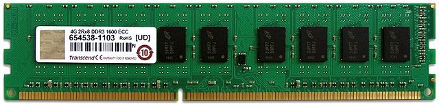
Modern DDR3 SDRAM. Source: BY-SA / 4.0 by Kjerish

During a recent visit to the Computer View Museum in Mountain View, my attention was drawn to an ancient sample of ferrite memory .


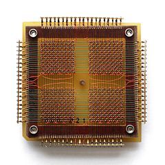
Source: BY-SA / 3.0 by Konstantin Lanzet

I quickly came to the conclusion that I have no idea how such things work. Do the rings rotate (no), and why three wires pass through each ring (I still don’t understand how they work). More importantly, I realized that I very poorly understand the principle of operation of modern dynamic RAM!
')

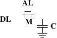
Source: Ulrich Drepper's Memory Cycle

I was particularly interested in one of the consequences of how dynamic RAM works. It turns out that every bit of data is stored by charge (or its absence) on a tiny capacitor in the RAM chip. But these capacitors gradually lose charge over time. To avoid losing stored data, they must be regularly updated to restore charge (if any) to the original level. This update process involves reading each bit, and then writing it back. In the process of such an "update", the memory is occupied and cannot perform normal operations, such as writing or storing bits.

It worried me for a long time, and I wondered ... can I notice a delay in updating at the program level?

Dynamic RAM Upgrade Training Base

Each DIMM consists of “cells” and “rows”, “columns”, “sides” and / or “ranks”. This presentation from the University of Utah explains the nomenclature. The configuration of the computer's memory can be checked with the decode-dimms . Here is an example:

  $ decode-dimms
 Size 4096 MB
 Banks x Rows x Columns x Bits 8 x 15 x 10 x 64
 Ranks 2 

We do not need to understand the whole DDR DIMM scheme, we want to understand the operation of only one cell storing one bit of information. Or rather, we are only interested in the update process.

Consider two sources:

• DRAM Update Tutorial from the University of Utah
• And Micron's excellent gigabit chip documentation: “Designing a TN-46-09 for 1Gb DDR SDRAM”

Every bit in the dynamic memory should be updated: it usually happens every 64 ms (the so-called static update). This is quite an expensive operation. To avoid one major stop every 64 ms, the process is divided into 8192 smaller update operations. In each of them, the computer memory controller sends update commands to the DRAM chips. After receiving the instructions, the chip will update 1/8192 cells. If you count, then 64 ms / 8192 = 7812.5 ns or 7.81 μs. This means the following:

• The refresh command is executed every 7812.5 ns. It is called tREFI.
• The update and restore process takes some time, so the chip can perform normal read and write operations again. The so-called tRFC is either 75 ns or 120 ns (as in the mentioned Micron documentation).

If the memory is hot (more than 85 ° C), then the storage time of the data in the memory drops, and the static update time is halved to 32 ms. Accordingly, the tREFI falls to 3906.25 ns.

A typical memory chip is busy updating for a considerable part of its work time: from 0.4% to 5%. In addition, the memory chips are responsible for the non-trivial share of the power consumption of a typical computer, and most of this power is spent on updating.

At the time of the update, the entire memory chip is blocked. That is, each bit in memory is locked for more than 75 ns every 7812 ns. Let's measure.

Preparing the experiment

To measure operations with nanosecond precision, we need a very dense cycle, perhaps at C. It looks like this:

  for (i = 0; i < ...; i++) { //   . *(volatile int *) one_global_var; //   CPU.    _mm_clflush(one_global_var); //   ,     //    (25    160). // , - . asm volatile("mfence"); //     clock_gettime(CLOCK_MONOTONIC, &ts); } 

The full code is available on github.

The code is very simple. We execute reading of memory. We reset the data from the CPU cache. We measure time.

(Note: in the second experiment, I tried to use MOVNTDQA to load data, but this requires a special non-cached memory page and root rights).

On my computer, the program gives the following data:

  # timestamp, cycle time
 3101895733, 134
 3101895865, 132
 3101896002, 137
 3101896134, 132
 3101896268, 134
 3101896403, 135
 3101896762, 359
 3101896901, 139
 3101897038, 137 

Usually a cycle of about 140 ns is obtained, periodically the time jumps to about 360 ns. Sometimes strange results are popping up more than 3200 ns.

Unfortunately, the data is too noisy. It is very difficult to see if there is a noticeable delay associated with update cycles.

Fast Fourier Transform

At some point it dawned on me. Since we want to find an event with a fixed interval, we can submit the data to the FFT algorithm (fast Fourier transform), which will decode the basic frequencies.

I’m not the first to think about this: Mark Seborn with the famous vulnerability Rowhammer implemented this very technique back in 2015. Even looking at the Mark code, making FFT work was harder than I expected. But in the end I put all the pieces together.

First you need to prepare the data. FFT requires input with a constant sampling interval. We also want to trim the data to reduce noise. Through trial and error, I found that the best result is achieved after preprocessing the data:

• Small values ​​(less than 1.8 average) loop iterations are cut off, ignored and replaced with zeros. We really don't want to introduce noise.
• All other readings are replaced by units, since we really do not care about the amplitude of the delay caused by some noise.
• I stopped at a sampling interval of 100 ns, but any number up to the Nyquist frequency (double expected frequency) will do .
• Data must be selected with a fixed time before submission to the FFT. All reasonable sampling methods work fine, I stopped at the basic linear interpolation.

Algorithm like this:

 UNIT=100ns A = [(timestamp, loop_duration),...] p = 1 for curr_ts in frange(fist_ts, last_ts, UNIT): while not(A[p-1].timestamp <= curr_ts < A[p].timestamp): p += 1 v1 = 1 if avg*1.8 <= A[p-1].duration <= avg*4 else 0 v2 = 1 if avg*1.8 <= A[p].duration <= avg*4 else 0 v = estimate_linear(v1, v2, A[p-1].timestamp, curr_ts, A[p].timestamp) B.append( v ) 

Which on my data produces a rather boring vector like this:

  [0, 0, 0, 0, 0, 0, 0, 0, 0, 0, 0, 0, 0, 0, 0, 0, 0, 0, 
  0, 0, 0, 0, 0, 0, 0, 0, 0, 0, 0, 0, 0, 0, 0, 1, 1, 0,
  0, 0, 0, 0, 0, 0, 0, 0, 0, 0, 0, 0, 0, 0, 0, 0, 0, 0, 
  0, 0, 1, 0, 0, 0, 0, 0, 0, 0, 0, 0, 0, 0, 0, 0, 0, 0, ...] 

However, the vector is quite large, usually about 200 thousand data points. With such data you can use FFT!

 C = numpy.fft.fft(B) C = numpy.abs(C) F = numpy.fft.fftfreq(len(B)) * (1000000000/UNIT) 

Pretty simple, right? It produces two vectors:

• C contains complex numbers of frequency components. We are not interested in complex numbers, and we can smooth them with the abs() command.
• F contains labels, which frequency interval lies in which place of the vector C. Normalize the parameter to Hertz by multiplying by the sampling rate of the input vector.

The result can be applied to the chart:



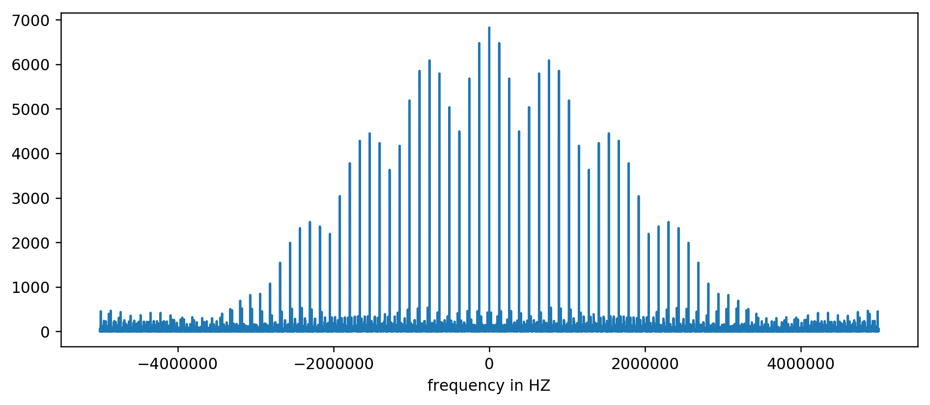
Y axis without units, since we normalized the delay time. Despite this, bursts are clearly visible in certain fixed frequency intervals. Consider them closer:



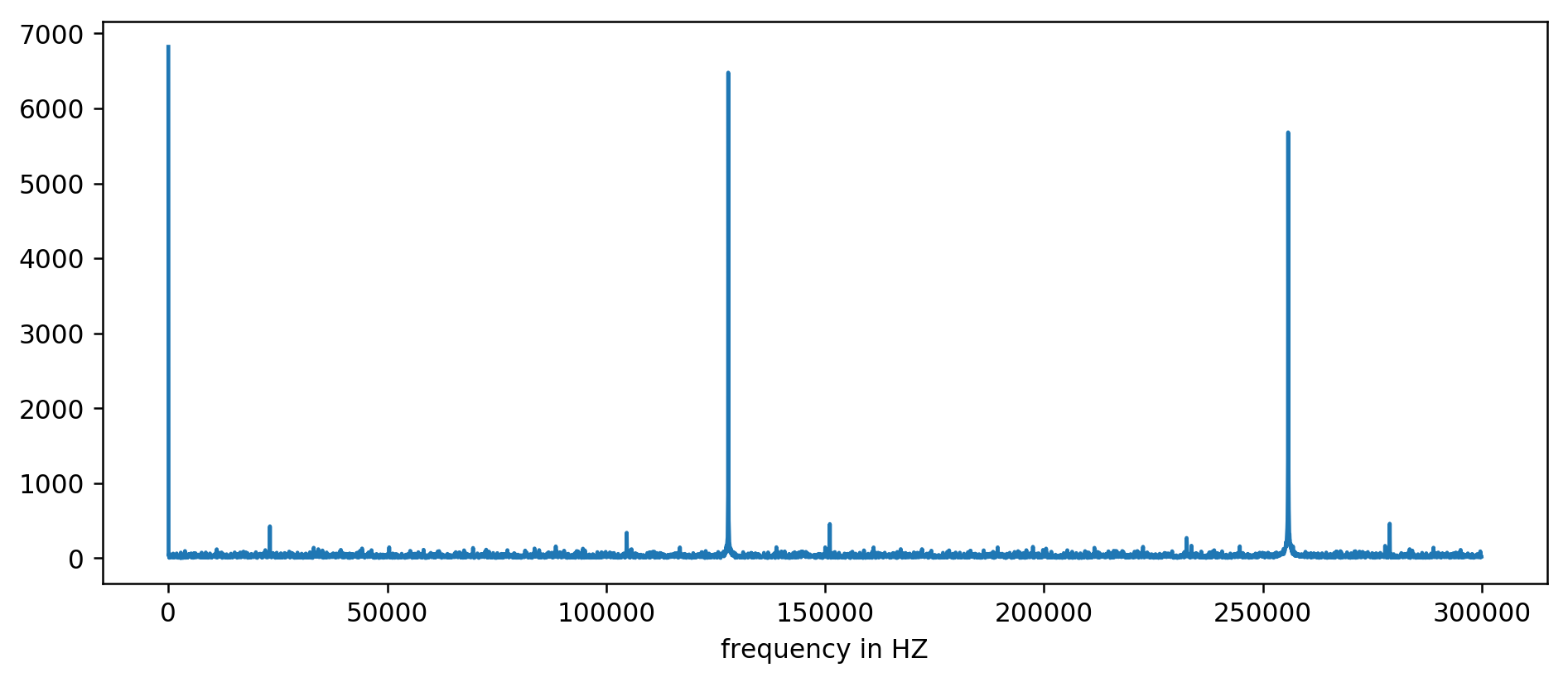
We clearly see the first three peaks. After a little inexpressive arithmetic, including filtering the reading at least ten times the size of the average, you can extract the base frequencies:

  127850.0
 127900.0
 127950.0
 255700.0
 255750.0
 255800.0
 255850.0
 255900.0
 255950.0
 383600.0
 383650.0 

We count: 1,000,000,000 (ns / s) / 1,27900 (Hz) = 7,818.6 ns

Hooray! The first frequency jump is really what we were looking for, and it really correlates with the update time.

The remaining peaks at 256 kHz, 384 kHz, 512 kHz are the so-called harmonics, multiples of our base frequency of 128 kHz. This is a completely expected side effect of using FFT on something like a square wave .

To facilitate experiments, we made a command line version . You can run the code yourself. Here is an example of running on my server:

  ~ / 2018-11-memory-refresh $ make
 gcc -msse4.1 -ggdb -O3 -Wall -Wextra measure-dram.c -o measure-dram
 ./measure-dram |  python3 ./analyze-dram.py
 [*] Verifying ASLR: main = 0x555555554890 stack = 0x7fffffefe22
 [] Fun fact.  I did 40663553 clock_gettime () 's per second
 [*] Measuring MOVQ + CLFLUSH time.  Running 131072 iterations.
 [*] Writing out data
 [*] Input data: min = 117 avg = 176 med = 167 max = 8172 items = 131072
 [*] Cutoff range 212-inf
 [] 127849 items below cutoff, 0 items above cutoff, 3223 items non-zero
 [*] Running FFT
 [*] Top frequency above 2kHz below 250kHz has magnitude of 7716
 [+] Top frequency spikes above 2kHZ are at:
 127906Hz 7716
 255813Hz 7947
 383720Hz 7460
 511626Hz 7141 

I have to admit, the code is not quite stable. In case of problems, it is recommended to disable Turbo Boost, CPU frequency scaling and performance optimization.

Conclusion

From this work there are two main conclusions.

We have seen that low-level data is rather difficult to analyze and seems rather noisy. Instead of evaluating with the naked eye, you can always use the good old FFT. In preparing the data, it is necessary in some sense to take what was desired.

Most importantly, we have shown that it is often possible to measure subtle hardware behavior from a simple process in user space. This kind of thinking led to the discovery of the original vulnerability of Rowhammer , it is implemented in the Meltdown / Specter attacks and again shown in the recent reincarnation of Rowhammer for ECC memory .

Much remains beyond the scope of this article. We barely touched the internal workings of the memory subsystem. For further reading, I recommend:

• L3 cache mapping on Sandy Bridge processors
• How a physical address is matched with strings and banks in DRAM
• Hanna Hartikainen cracked DDR3 SO-DIMM and made him work ... slower

Finally, here is a good description of old ferrite memory:

• Explanation of ferrite memory PDP-11 from the University of Sydney