There are a number of tasks in which the time-consuming signal is divided into segments, each of which is processed separately. In particular, this approach is used to analyze the signal using the window Fourier transform, or vice versa, during synthesis; as well as spectral processing such as noise removal, tempo changes, nonlinear filtering, audio data compression, and others.

The splitting process itself is mathematically represented by multiplying by some weight ( window ) function with offset. For the simplest window — rectangular — it might look like this:

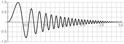
Source signal:
')


Splits:







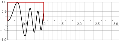
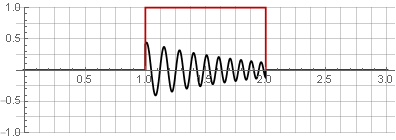
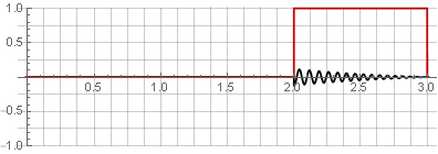
You can restore the original signal by simply summing them up.

Read more

However by For some reasons, a rectangular function is not the best window function. When spectral analysis through the (usually fast) discrete Fourier transform, the analyzed data block “loops”, as it were, which leads to rupture at the edges and distortion of the spectrum:



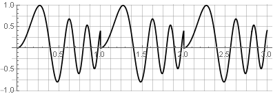
It is not suitable for reverse synthesis - since any change will also lead to discontinuities - for example, if we try to reverse one of the parts:



To eliminate these shortcomings, overlapping is used - when each next window captures part of the data from the previous one; and the weight window, respectively, smoothly falls to the edges.

50% overlap

The most common use for this is the Hanna window (also known as the “raised cosine”) with an overlap of 50%:








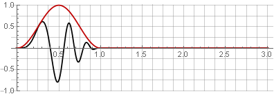
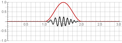
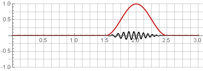
Due to the symmetry of the cosine function when added, they are summed to one:



Now, in the reverse synthesis, we will not get discontinuities - but only under the condition that the values ​​at the window borders will still go to zero. For example, when reversing one of the parts, the smoothness is not disturbed:

Processing double overlay windows

Let us consider in more detail the algorithm for signal processing using the fast Fourier transform (FFT):

1. splitting the signal into segments with overlapping window;
2. direct FFT;
3. spectrum processing;
4. reverse FFT;
5. repeated overlapping of the window (since after the inverse FFT the boundaries will not necessarily be joined to zero without a break);
6. summation of the resulting segments.

At the same time, if spectrum processing is not performed, the output signal must be identical to the input signal (only with the inevitable time delay).

When using the Hanna window, overlapping by 50% is no longer enough, since failures will occur:



Since double overlap is tantamount to squaring, the obvious solution would be to use the root from the Hanna window to compensate for squaring:



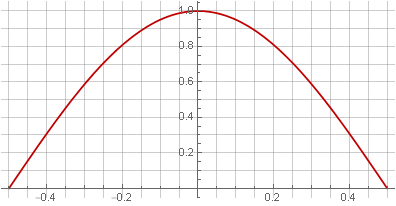
In this case, however, the window ceased to be smooth at the edges - a gap appeared in the first derivative.


You can go the other way - to use the overlap of 75%, and then the windows will also be added to a constant - just not in $$$1$ and in $$$\ frac {3} {2}$ :



In this case, we just got lucky. If we decompose a square into an amount, we can see that it is a composition of two Hanna windows, but at different scales, which allows us to fulfill the requirements we need:

$$

$$\ left (\ frac {\ cos (2 \ pi x) +1} {2} \ right) ^ 2 = \ frac {\ cos (2 \ pi x) +1} {2} + \ frac {\ cos (4 \ pi x) -1} {8}$$

With other window functions, such a focus will not work; Also, not all standard window functions can provide summation in a constant and at 50% overlap.

Idea

You can consider the Hanna window not as an independent function, but as the difference between two piecewise-continuous functions (a separate article was devoted to detailed consideration) with an offset. For example, using the following function

$$

$$\ left \ {\ begin {array} {ll} -1 & x \ leqslant -1 \\ 1 & x \ geqslant 1 \\ \ sin \ left (\ frac {\ pi x} {2} \ right) & -1 <x <1 \\ \ end {array} \ right.$$

can write

$$

$$f (x + 1) -f (x-1)$$

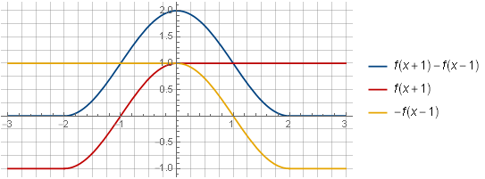
Having considered the components of the sum of two such windows, their ability to add up to a constant will become more intuitive:



On the segment $$$[0,2]$ we received mutual compensation when adding functions $$$-f (x-1)$ and $$$f ((x + 1) -2)$ , insofar as $$$f ((x + 1) -2) = f (x-1)$

You can also select another offset, with a large overlap, for example:

$$

$$f \ left (x + \ frac {1} {2} \ right) -f \ left (x- \ frac {1} {2} \ right)$$

And then, when offset in increments $$$\ frac {1} {2}$ , they will also be added to a constant:



It can be seen that if you rearrange the components of the window function, you get all the same windows Hannah.

Thus, using various functions of restriction, it is possible to form windows of the necessary form.

Final formula

Now it only remains to set the scale so that the definition areas and values ​​do not depend on the amount of overlap. Defining a window on the interval $$$[0,1]$ will get

$$

$$\ frac {f \ left (\ frac {2 tx} {t-1} -1 \ right) -f \ left (\ frac {2 t (x-1)} {t-1} +1 \ right) } {2}$$

Where $$$f$ - piecewise continuous form function

$$

$$\ left \ {\ begin {array} {ll} -1 & x \ leqslant -1 \\ 1 & x \ geqslant 1 \\ g (x) & -1 <x <1 \\ \ end {array} \ right.$$

but $$$g$ - some interpolating function between points $$$(- 1, -1)$ and $$$(1,1)$ .

Parameter $$$t$ determines the level of overlap - the divisor that determines the step to which each next window should be shifted, $$$x_ {n + 1} = x_n + \ frac {1} {t}$ , and must be greater than one, $$$t> 1$ .

Overlap percentage $$$p$ can be calculated by the formula

$$

$$p = \ frac {100 (t-1)} {t}$$

and vice versa

$$

$$t = \ frac {100} {100-p}$$

The final view of the window will depend on both the choice of the level of overlap and the choice of the limiting function.

Some interesting examples

Here we look at several ready-made solutions for which everything was started. For simplicity, we will consider just the interpolating function. $$$g (x)$ without any other strapping.

Polynomial windows

They are the least computationally expensive. Using the previously derived formula

$$

$$\ frac {2 x \ Gamma \ left (n + \ frac {1} {2} \ right) \, _2F_1 \ left (\ frac {1} {2}, 1-n; \ frac {3} {2} ; x ^ 2 \ right)} {\ sqrt {\ pi} \ Gamma (n)}$$

we obtain a polynomial with a given number of zeros on higher derivatives that provide the necessary smoothness of the window at the edges.


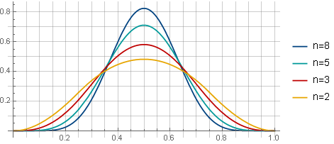
With a 75% overlap, windows with different values ​​of n will look like this:



And in the case of root extraction, this is the case (using 75% overlap):



or so (when using 50% overlap):

Maximum smooth window

Function

$$

$$\ tanh \ left (\ frac {k x} {\ sqrt {1-x ^ 2}} \ right)$$

It is interesting in that it is infinitely differentiable and all its derivatives at the edges are 0 (which can be proved by considering its derivatives based on the rules of differentiation - in each term there will be a multiplying factor). This allows building windows on its basis, all derivatives of which have no discontinuities:

Window "skirt"

The need for this type of window is caused by increasing the resolution of the FFT, but reducing the effect of the “time-frequency uncertainty” effect at high frequencies by increasing their concentration in the center.

First, we define the desired type of window function - for example, as follows:

$$

$$- \ log \ left (k ^ 2 x ^ 2 + 1 \ right) + \ log \ left (k ^ 2 + 1 \ right) - \ frac {k ^ 2 \ left (1-x ^ 2 \ right) } {k ^ 2 + 1}$$

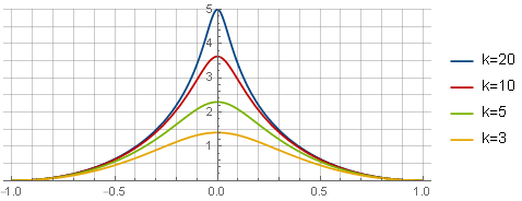
Here, the first term determines the type of the function itself, the second one provides the intersection with the abscissa axis, the third (parabola) nullifies the derivative at the edges for a smooth docking; and the parameter $$$k$ defines the "sharpness" of the top. In this form, it is not yet suitable for use - first, it is necessary to obtain the function of restriction from it through integration and scaling:

$$

$$\ frac {kx \ left (k ^ 2 \ left (x ^ 2 + 3 \ right) + 6 \ right) +3 \ left (k ^ 2 + 1 \ right) \ left (kx \ left (\ log \ left (k ^ 2 + 1 \ right) - \ log \ left (k ^ 2 x ^ 2 + 1 \ right) \ right) -2 \ tan ^ {- 1} (kx) \ right)} {4 k ^ 3-6 \ left (k ^ 2 + 1 \ right) \ tan ^ {- 1} (k) +6 k}$$

For convenience, you can bind the parameter $$$k$ overlap level $$$t$ - for example, so that the 4th derivative in the center of the window was 0 - and then $$$k$ will be counted as $$$\ sqrt {3} (t-1)$ :



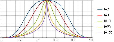
Here, for clarity, all windows are reduced to the same scale.

Window view "needle"

It is a more "aggressive" version of the previous window. As a basis, a hyperbola was chosen, from which, by successive transformations

$$

$$\ frac {1} {x} \ to \ frac {1} {\ sqrt {x ^ 2}} \ to \ frac {1} {\ sqrt {x ^ 2 + 1}} \ to \ frac {1} {\ sqrt {k ^ 2 x ^ 2 + 1}} \ to \ frac {\ left (1-x ^ 2 \ right) ^ 2} {\ sqrt {k ^ 2 x ^ 2 + 1}}$$

and using the same steps in the form of integration and scaling we got the formula

$$

$$\ frac {kx \ left (2 k ^ 2 \ left (x ^ 2-4 \ right) -3 \ right) \ sqrt {k ^ 2 x ^ 2 + 1} + \ left (8 \ left (k ^ 4 + k ^ 2 \ right) +3 \ right) \ sinh ^ {- 1} (kx)} {\ left (8 \ left (k ^ 4 + k ^ 2 \ right) +3 \ right) \ sinh ^ {-1} (k) -3 k \ sqrt {k ^ 2 + 1} \ left (2 k ^ 2 + 1 \ right)}$$

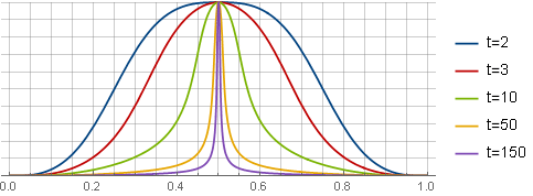
Here you can also bind the parameter $$$k$ to the level of overlap. Directly solving the 4th derivative equation is too cumbersome, so we’ll just make the solution for the previous window in the same way as $$$k$ as $$$k (t-1)$ thus ensuring the role of the parameter $$$k$ as “fine tuning”. With $$$k = 2.22$ windows will look like this:

Asymmetrical window

The window function does not necessarily have to be symmetrical. Suppose we need a window with a sharp attack and a smooth attenuation. We can get it according to the already familiar scheme - first determine the desired type of function, and then integrate to get the restriction function. Here, the task is slightly complicated due to the fact that, due to asymmetry, the center will no longer pass through the origin, therefore an additional calculation step is added. This also leads to the fact that the formulas as a result are quite cumbersome. For example, consider the simplest option - a parabola multiplied by a polynomial weight window:

$$

$$(1-x) ^ 2 \ left (1-x ^ {10} \ right) ^ 2$$

Here, the degree at x in the weighted window (namely, 10) determines the “sharpness” of the attack. We used a specific value, rather than a character parameter, to simplify the formulas for clarity - if you wish, you can recalculate it later.

After integration, just scaling is no longer enough - you need to even out the edges:



To do this, we first move the function to the top to align the left edge, and then scale it to the right along the two and subtract one. Then we get the following formula:

$$

$$\ frac {8775 \ left (\ frac {x ^ {27}} {27} - \ frac {2 x ^ {26}} {26} + \ frac {x ^ {25}} {25} - \ frac {2 x ^ {15}} {15} + \ frac {4 x ^ {14}} {14} - \ frac {2 x ^ {13}} {13} + \ frac {x ^ 3} {3} -x ^ 2 + x + \ frac {117592} {61425} \ right)} {9856} -1$$

In order for the final window to have the desired appearance, it is also necessary to ensure a sufficiently large level of overlap:

Conclusion

Similarly, windows can be constructed from any other bell-shaped functions — for example, Gaussians; and it is also possible to modify those already considered in order to provide greater smoothness or change in the shape of the curve.

The spectral composition of such window functions has remained outside of consideration — separate studies should be devoted to this.

A slightly more advanced version of the article (with the ability to dynamically change the parameters in the windows under consideration and hidden formulas) as a Wolfram Mathematica document can be downloaded here .