Trading robot optimization algorithms: an effective way to trade a million in hindsight
I read an authoritative book on trading strategies and wrote my trading robot. To my surprise, the robot does not bring millions, even trading virtually. The reason is obvious: a robot, like a racing car, needs “tuning”, in the selection of parameters adapted to a specific market, a specific period of time.
Since the robot has enough settings, it is time consuming to sort through all their possible combinations in search of the best, too time consuming. At one time, while solving an optimization problem, I did not find an informed choice of the search algorithm for a quasi-optimal vector of parameters of a trading robot. Therefore, I decided to independently compare several algorithms ...
Brief formulation of the optimization problem
We have a trading algorithm. Input data - price history of the hourly interval for 1 year of observations. Output - P - profit or loss, a scalar value.
')
The trading algorithm has 4 custom parameters:
- Mf is the “fast” moving average period,
- Ms period of the “slow” moving average
- T - TakeProfit, the target profit level for each individual transaction,
- S - StopLoss, target loss level for each individual transaction.
We assign a range and a fixed step of change to each of the parameters, a total of 20 values for each of the parameters.
Thus, we can search for the maximum profit (P) for one parameter on one array of input data:
- varying one parameter, for example, P = f (Ms), producing up to 20 backtests ,
- varying two parameters, for example, P = f (Ms, T), producing up to 20 * 20 = 400 backtests,
- varying three parameters, for example P = f (Mf, Ms, T), producing up to 20 * 20 * 20 = 8,000 backtests,
- varying each of the parameters, P = f (Mf, Ms, T, S) and performing up to 20 ^ 4 = 160,000 backtests.
For most trading algorithms, however, it takes several orders of magnitude more time to conduct a single test. Which leads us to the task of finding a quasi-optimal vector of parameters without having to search through the whole set of possible combinations of them.
in detail about trade and trading robots
Trading on the stock exchange, betting in the Forex dealing center, crazy betting on “binary options”, cryptocurrency speculation - a kind of “diagnosis”, with several possible options for the development of the “disease”. A very common scenario is when a player, having played with “intuition”, comes to automatic trading. Do not misunderstand me, I don’t want to put such accents in such a way that “technologically and mathematically” strict trading robots are opposed to naive and helpless “manual” trading. For example, I myself am convinced that any of my attempts to extract from an efficient market (read from any transparent and liquid market) profits through speculation, whether discretionary or fully automated, are a priori doomed to failure. If, perhaps, to prevent the factor of accidental luck.
Nevertheless, trading, and, in particular, algo (rhythmic) trading is a popular hobby for many. Some program their own trading robots, others go even further and create their own platforms for writing, debugging and backtesting trading strategies, and others download / buy a ready-made electronic “expert”. But even those who do not write the trading algorithms on their own should have an idea of how to handle this “black box” in order to extract profit from it in accordance with the author's idea. In order not to be unfounded, I present my further observations on the example of a simple trading strategy:
The trading robot analyzes the price of gold, in dollars per troy ounce, and decides whether to buy or sell a certain amount of gold. For simplicity, we assume that the robot always trades one troy ounce.
For example, at the time of purchase, the cost of an ounce of gold was 1075.00 USD . At the time of the subsequent sale (closing of the transaction) the price increased to 1079.00 USD. Profit for this transaction amounted to 4 USD.
If the robot “sold” gold at 1075.00 USD, and subsequently completed (closed) the transaction, “having bought” gold back at a price of 1079 USD, the profit on the transaction will be a negative value - minus 4 USD. Actually, for us it does not matter how the robot sells gold, which it does not have, in order to “buy back” it back. Broker / dealing center allows a trader to “buy” and “sell” an asset in one way or another, earning (or, more often, losing) the difference in rates.
With the input data for the robot, we decided - this is, in fact, the time series of prices (quotations) of gold. If you say that my example is too simple, not vital, I can assure you: most of the robots traded on the market (and the traders themselves too) are guided in their trade only by the statistics of prices for the goods they trade. In any case, in the problem of parametric optimization of a trading strategy, there is no fundamental difference between a robot trading on the basis of a price vector and a robot accessing a terabyte array of multi-market analytics. The main thing is that both of these robots can (should be able to) be tested on historical data. Algorithms must be deterministic: that is, on the same input data (model time, if necessary, we can also take it as a parameter), the trading robot must show the same result.
Nevertheless, trading, and, in particular, algo (rhythmic) trading is a popular hobby for many. Some program their own trading robots, others go even further and create their own platforms for writing, debugging and backtesting trading strategies, and others download / buy a ready-made electronic “expert”. But even those who do not write the trading algorithms on their own should have an idea of how to handle this “black box” in order to extract profit from it in accordance with the author's idea. In order not to be unfounded, I present my further observations on the example of a simple trading strategy:
Simple trading robot
The trading robot analyzes the price of gold, in dollars per troy ounce, and decides whether to buy or sell a certain amount of gold. For simplicity, we assume that the robot always trades one troy ounce.
For example, at the time of purchase, the cost of an ounce of gold was 1075.00 USD . At the time of the subsequent sale (closing of the transaction) the price increased to 1079.00 USD. Profit for this transaction amounted to 4 USD.
If the robot “sold” gold at 1075.00 USD, and subsequently completed (closed) the transaction, “having bought” gold back at a price of 1079 USD, the profit on the transaction will be a negative value - minus 4 USD. Actually, for us it does not matter how the robot sells gold, which it does not have, in order to “buy back” it back. Broker / dealing center allows a trader to “buy” and “sell” an asset in one way or another, earning (or, more often, losing) the difference in rates.
With the input data for the robot, we decided - this is, in fact, the time series of prices (quotations) of gold. If you say that my example is too simple, not vital, I can assure you: most of the robots traded on the market (and the traders themselves too) are guided in their trade only by the statistics of prices for the goods they trade. In any case, in the problem of parametric optimization of a trading strategy, there is no fundamental difference between a robot trading on the basis of a price vector and a robot accessing a terabyte array of multi-market analytics. The main thing is that both of these robots can (should be able to) be tested on historical data. Algorithms must be deterministic: that is, on the same input data (model time, if necessary, we can also take it as a parameter), the trading robot must show the same result.
In more detail about the trading robot it is possible to read in the following spoiler:
robot trading algorithm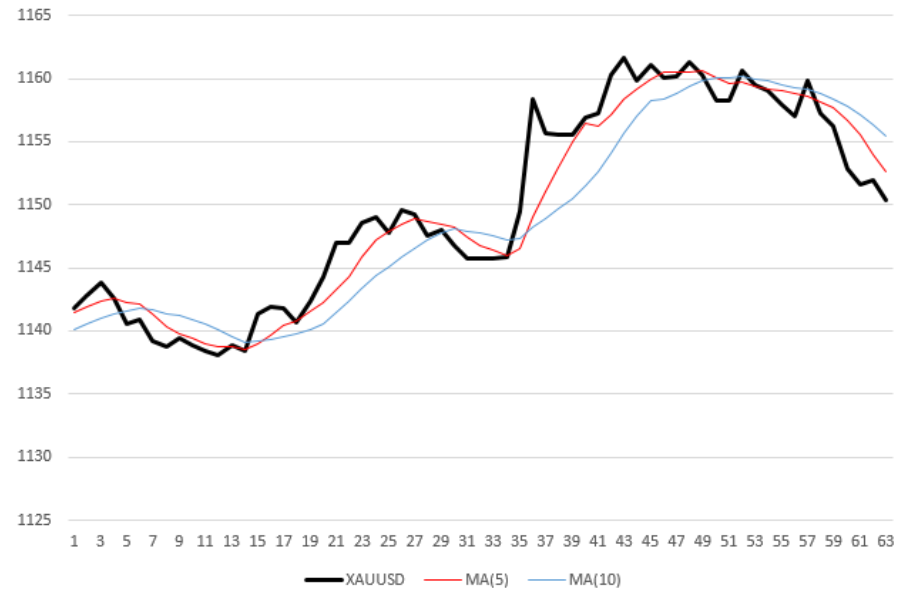
The black (thick) curve on the chart is the hourly XAUUSD price measurements. Two thin broken lines, red and blue - averaged price values with averaging periods of 5 and 10, respectively. In other words, moving averages (Moving Average, MA) with periods of 5, 10. For example, in order to calculate the ordinate of the last (right) point of the red curve, I took the average of the last 5 price values. Thus, each moving average is not only “smoothed” relative to the price curve, but also lags behind it by half of its period.
The robot has a simple rule for making a purchase / sale decision:
- as soon as the moving average with a short period (“fast” MA ) crosses the moving average with a long period (“slow” MA) from the bottom up, the robot buys the asset (gold).
As soon as the “fast” MA crosses the “slow” MA from top to bottom, the robot sells the asset. In the picture above, the robot will make 5 transactions: 3 sales in time stamps 7, 31 and 50, and two purchases (marks 16 and 36).
The robot is allowed to open an unlimited number of transactions. For example, at some point the robot may have several pending purchases and sales at the same time.
The robot closes the deal as soon as:
Suppose StopLoss is 0.2%.
The deal is a “sale” of gold at a price of 1061.50.
As soon as the price of gold rises to the value of 1061.50 + 1061.50 * 0.2% / 100% = 1063.12%, the loss on the transaction will obviously be equal to 0.2% and the robot will close the transaction automatically.
The robot makes all decisions on opening / closing a deal at discrete points in time - at the end of each hour, after the publication of the next XAUUSD quote.
Yes, the robot is extremely simple. At the same time, it is 100% compliant with the requirements for it:
On the example of our simple robot, it is clear that a complete enumeration of all possible vectors of robot settings is too expensive, even for 4 variable parameters. An obvious alternative to complete enumeration is the choice of parameter vectors according to a certain strategy. We consider only a part of all possible combinations in search of the best, in which the GF approaches the highest (or the smallest, depending on which GF we chose and what result we achieve) value.
The black (thick) curve on the chart is the hourly XAUUSD price measurements. Two thin broken lines, red and blue - averaged price values with averaging periods of 5 and 10, respectively. In other words, moving averages (Moving Average, MA) with periods of 5, 10. For example, in order to calculate the ordinate of the last (right) point of the red curve, I took the average of the last 5 price values. Thus, each moving average is not only “smoothed” relative to the price curve, but also lags behind it by half of its period.
Open transaction rule
The robot has a simple rule for making a purchase / sale decision:
- as soon as the moving average with a short period (“fast” MA ) crosses the moving average with a long period (“slow” MA) from the bottom up, the robot buys the asset (gold).
As soon as the “fast” MA crosses the “slow” MA from top to bottom, the robot sells the asset. In the picture above, the robot will make 5 transactions: 3 sales in time stamps 7, 31 and 50, and two purchases (marks 16 and 36).
The robot is allowed to open an unlimited number of transactions. For example, at some point the robot may have several pending purchases and sales at the same time.
Closing Rule
The robot closes the deal as soon as:
- profit on the transaction exceeds the threshold specified in percent - TakeProfit,
- or the loss on the transaction, as a percentage, exceeds the corresponding value - StopLoss.
Suppose StopLoss is 0.2%.
The deal is a “sale” of gold at a price of 1061.50.
As soon as the price of gold rises to the value of 1061.50 + 1061.50 * 0.2% / 100% = 1063.12%, the loss on the transaction will obviously be equal to 0.2% and the robot will close the transaction automatically.
The robot makes all decisions on opening / closing a deal at discrete points in time - at the end of each hour, after the publication of the next XAUUSD quote.
Yes, the robot is extremely simple. At the same time, it is 100% compliant with the requirements for it:
- the algorithm is determined: each time, imitating the work of the robot on the same price data, we will get the same result,
- has a sufficient number of adjustable parameters, and specifically: the “fast” period and the “slow” moving average period (natural numbers), TakeProfit and StopLoss are positive real numbers,
- the change of each of the 4 parameters, in general, has a non-linear effect on the characteristics of the trade of the robot, in particular, on its profitability,
- the profitability of the robot on price history is considered to be an elementary program code, and the calculation itself takes a fraction of a second for a vector of one thousand quotations,
- Finally, that, however, is irrelevant, the robot, for all its simplicity, will in reality prove itself no worse (albeit, probably not better) than the Grail, sold by the author on the Internet for an immodest sum.
Quick search for a quasi-optimal set of input parameters
On the example of our simple robot, it is clear that a complete enumeration of all possible vectors of robot settings is too expensive, even for 4 variable parameters. An obvious alternative to complete enumeration is the choice of parameter vectors according to a certain strategy. We consider only a part of all possible combinations in search of the best, in which the GF approaches the highest (or the smallest, depending on which GF we chose and what result we achieve) value.
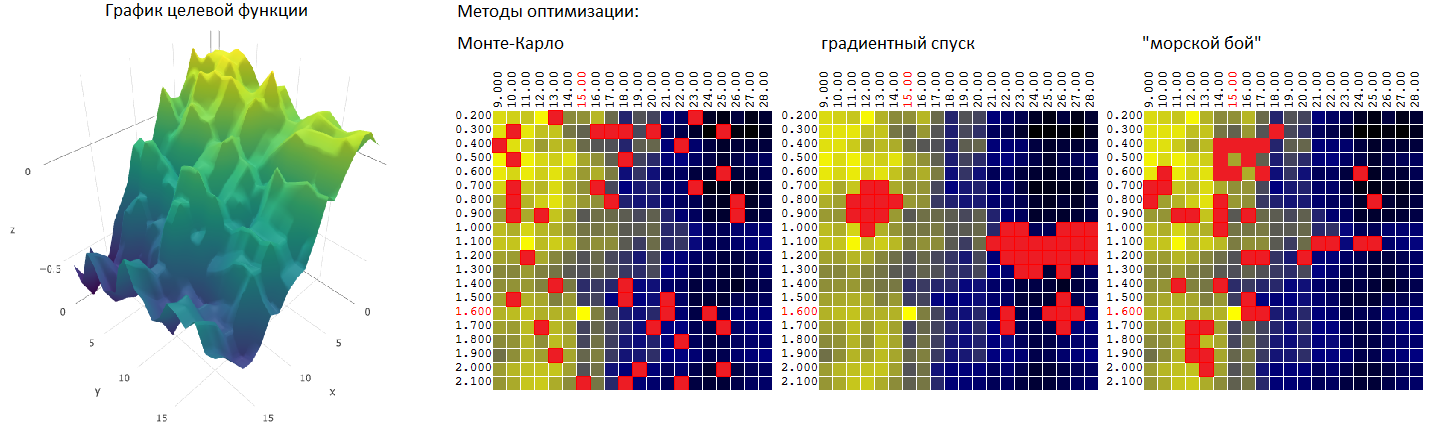
We consider three algorithms for finding the quasi- optimal value of the FC . For each algorithm, we set a limit of 40 tests (out of 400 possible combinations).
Monte Carlo method
or a random selection of M uncorrelated vectors from among the possible number of sets equal to N. The method is probably the simplest possible one. We will use it as a starting point for later comparison with other optimization methods.
Example 1
the graph shows the dependencies of the profit (P) of our trading robot, trading EURUSD , obtained at the annual segment of the history of hourly price measurements, on the value of the parameter - the period of the “slow” moving average (M). All other parameters are fixed and not optimized.
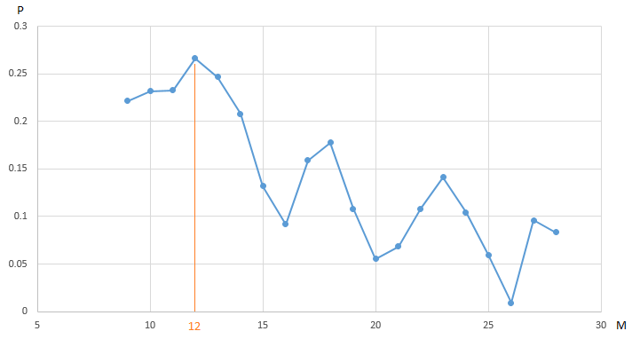
CF (profit) reaches a maximum of 0.27 at the point M = 12. To ensure that we find the maximum value of profit, we need to spend 20 test iterations. The alternative is to conduct a smaller number of tests of a trading robot with a randomly chosen value of the parameter M in the interval [9, 20]. For example, after 5 iterations (20% of the total number of tests, we found a quasi-optimal vector (a vector, obviously, one-dimensional) parameters: M = 18 with a DF value (M) equal to 0.18:

The remaining values on the graph from our optimization algorithm hid the “fog of war”.
Optimization of one of the four parameters of our trading robot, with fixed values of the other parameters, does not allow us to see the whole picture. Perhaps the maximum GF of 0.27 is not the best value of the indicator, if you vary the value of other parameters?

This is how the dependence of the profit on the moving average period changes for different values of the TakeProfit parameter in the interval [0.2 ... 0.8].
Monte Carlo method: optimization of two parameters
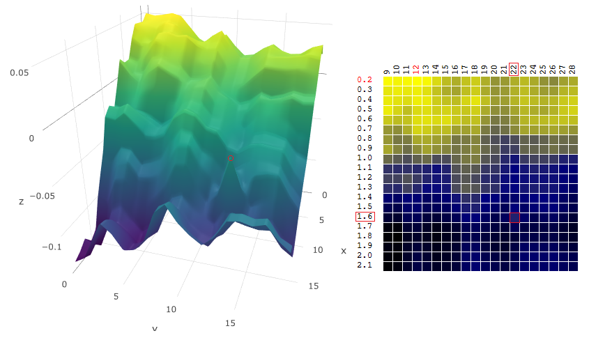
The dependence of the profit of a trading robot on two parameters can be graphically depicted as a surface:

The values of the parameters T (TakeProfit) and M (moving average period) are plotted along two axes, the third axis is the value of profit.
For our trading robot, after conducting 400 tests on a data interval of one year (~ 6000 hourly quotes of euro to US dollar), we obtain the surface of the form:

or, on the plane, where the values of TF (profit, P) are represented by color:

Choosing arbitrary points on the plane, in this example, the algorithm did not find the optimal value, but got close enough to it:

How effective is the Monte Carlo method in finding the maximum of the FIT ? After 1,000 iterations of searching for the maximum of the FF on the source data from the example above, I obtained the following statistics:
- the average value of the maximum of the functional phase found during 1,000 iterations of optimization (40 random vectors of parameters [M, T] of 400 possible combinations) was 0.231 or 95.7% of the global maximum of the functional phase (0.279).
Obviously, in comparing the methods of parametric optimization of trading robots, one sample is not an indicator. But for now this evaluation is enough. We proceed to the next method - the method of gradient descent .
Gradient descent method
Formally, as the name implies, the method is used to search for the minimum of the TF.
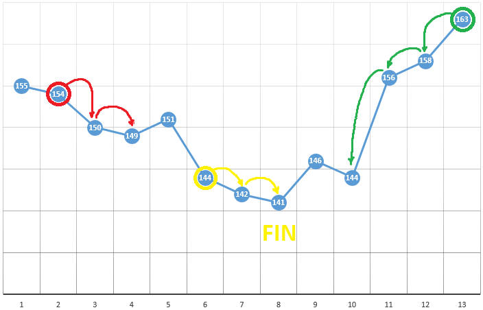
According to the method, we choose a starting point with coordinates [x0, y0, z0, ...]. Using the example of optimizing one parameter, this can be a randomly selected point:
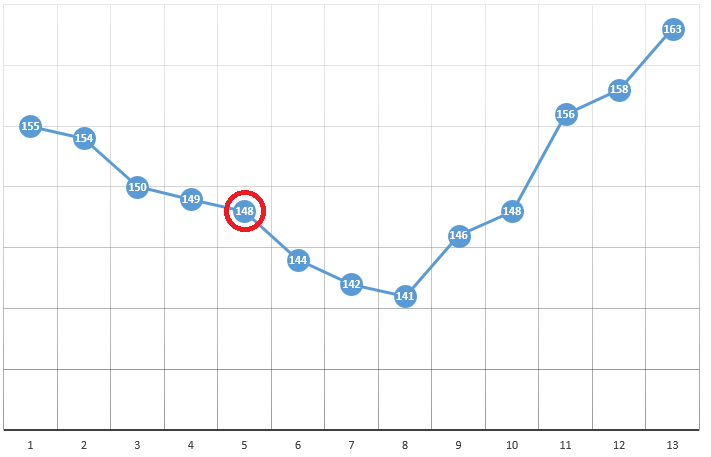
with coordinates [5] and TF value equal to 148. Next follow three simple steps:
- check the values of the GF in the vicinity of the current position (149 and 144)
- move to the point with the smallest ZF value
- if such is absent, a local extremum is found, the algorithm is completed

To optimize the CF as a function of two parameters, we use the same algorithm. If earlier we calculated CF in two adjacent points , now we check 4 points:
The method is definitely good when there is only one extremum in the TF of the test space. If there are several extremes, the search will have to be repeated several times to increase the probability of finding a global extremum:
In our example, we are looking for the maximum ZF. In order to remain within the framework of the definition of the algorithm, we can assume that we are looking for a minimum “minus CF”. The same example, the profit of a trading robot as a function of the period of the moving average and the TakeProfit value, is one iteration:
In this case, a local extremum was found, which is far from the global maximum of FC. An example of several iterations of finding the extremum of the CF by the method of gradient descent, the value of the CF is calculated 40 times (40 points out of 400 possible):

Now let's compare the efficiency of searching for the global maximum of the CF (profit) on our source data using Monte Carlo algorithms and gradient descent. In each case, 40 tests are carried out (calculations of ZF). 1,000 optimization iterations were performed by each of the methods:
| Monte Carlo | gradient descent | |
|---|---|---|
| the average of the obtained quasi-optimal value of the ZF | 0.231 | 0.200 |
| the obtained value of the maximum FC | 95.7% | 92.1% |
As we can see from the table, in this example, the gradient descent method does its job worse — finding the global extremum of the TF — the maximum profit. But not in a hurry to dismiss it.
Parametric stability of the trading algorithm
Finding the coordinates of the global maximum / minimum CF is often not the goal of optimization. Suppose there is a “sharp” peak on the graph - a global maximum, the value of the CF in the vicinity of which is significantly lower than the peak value:
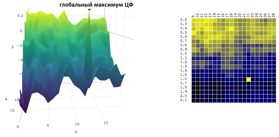
Suppose we chose the settings of the trading robot that match the found maximum of the ZF. If we slightly change the value of at least one of the parameters - the period of the moving average and / or TakeProfit - the profitability of the robot will fall sharply (will become negative). With regard to real trading, one can, at a minimum, expect that the market in which our robot is to trade will differ significantly from the period of history in which we optimized the trading algorithm.
Consequently, when choosing the “optimal” settings of a trading robot, it is worth getting an idea of how sensitive the robot is to changes in settings in the vicinity of the found extremum point of the ZF.
Obviously, the gradient descent method, as a rule, gives us the FF values in the vicinity of the extremum. The Monte Carlo method, rather, beats on the squares.
In multiple instructions for testing automated trading strategies, it is recommended that, after completing the optimization, check the target indicators of the robot in the vicinity of the parameter vector found. But these are additional tests. In addition, what if the profitability of the strategy falls with a slight change in settings? Obviously, you have to repeat the testing process.
An algorithm that, simultaneously with the search for the extremum of the FC, would allow us to assess the stability of the trading strategy to change the settings in a narrow range relative to the peaks found would be useful. For example, do not directly search for the maximum ZF
and the weighted average value, taking into account the neighboring values of the objective function, where the weight is inversely proportional to the distance to the neighboring value (to optimize the two parameters x, y and the objective function P):
In other words, when choosing a quasi-optimal vector of parameters, the algorithm will evaluate the “smoothed” objective function:
It was
has become
“Sea battle” method
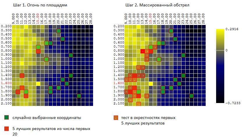
Trying to combine the advantages of both methods (Monte-Carlo and the gradient descent method), I tried an algorithm similar to the “sea battle” algorithm:
- At first I put several “blows” on the whole area.
- then, in places of “hits”, I open massive fire.
In other words, the first N tests are carried out on random uncorrelated vectors of input parameters. Of these, M best results are selected. In the vicinity of these tests (plus - minutes 0..L to each of the coordinates) another K test is being conducted.
For our example (400 points, 40 tests in total) we have:
Again, let's compare the effectiveness of now 3 optimization algorithms:
| Monte Carlo | gradient descent | “Sea battle” | |
|---|---|---|---|
| The average value of the found extremum of the TF as a percentage of the global value. 40 tests, 1,000 iterations of optimization | 95.7% | 92.1% | 97.0% |
The result is encouraging. Of course, the comparison was made on one specific data sample: one trading algorithm on one time series of the value of the euro against the US dollar. But, before comparing algorithms on more samples of source data, I am going to talk about another, unexpectedly (unjustifiably?) Popular algorithm for optimizing trading strategies - the genetic optimization algorithm (GA). However, the article was too voluminous, and the GA will have to be postponed for the next publication .
Source: https://habr.com/ru/post/430134/
All Articles