Data Science project from research to implementation on the example of Talking Hat

A month ago, Lenta launched a contest in which the same Talking Hat from Harry Potter determines who gave access to the social network of participants to one of the four faculties. The competition is not bad, the names sounding differently are determined by different faculties, and similar English and Russian names and surnames are distributed in a similar way. I don’t know if the distribution depends only on the names and surnames, and whether the number of friends or other factors is taken into account, but this contest prompted the idea of ​​this article: try to teach a classifier from scratch that will allow distributing users to different faculties.

In the article we will make a simple ML-model, which distributes people to the Harry Potter faculties, depending on their first and last name, going through a small research process following the CRISP methodology. Namely, we:

• We formulate the problem;
• We investigate possible approaches to its solution and formulate data requirements (Solution methods and data);
• Collect the necessary data (Solution methods and data);
• Explore assembled dataset (Exploratory Research);
• Extract features from raw data (Feature Engineering);
• We will train a model of machine learning (Model evaluation);
• Let's compare the obtained results, evaluate the quality of the solutions obtained and, if necessary, repeat paragraphs 2-6;
• We pack the solution into a service that can be used (Production).

This task may seem trivial, so we will impose an additional restriction on the whole process (so that it takes less than 2 hours) and on this article (so that its reading time is less than 15 minutes).

If you are already immersed in the wonderful and wonderful world of Data Science and Kagglit is constantly no one sees, or (God forbid) you like to measure your Hadup’s length during meetings with colleagues, then the article will most likely seem simple and uninteresting. Moreover, the quality of the final models is not the main value of this article. We warned you. Go.

For curious readers, a githab repository is also available with the code used in the article. In case of errors, please open the PR.

Formulate the task

Solving a problem that does not have clear decision criteria can be infinitely long, so we immediately decide that we want a solution that would allow us to get the answer “Gryffindor”, “Kogtevran”, “Puffenduy” or “Slytherin” in response to the entered string.

Essentially, we want a black box:

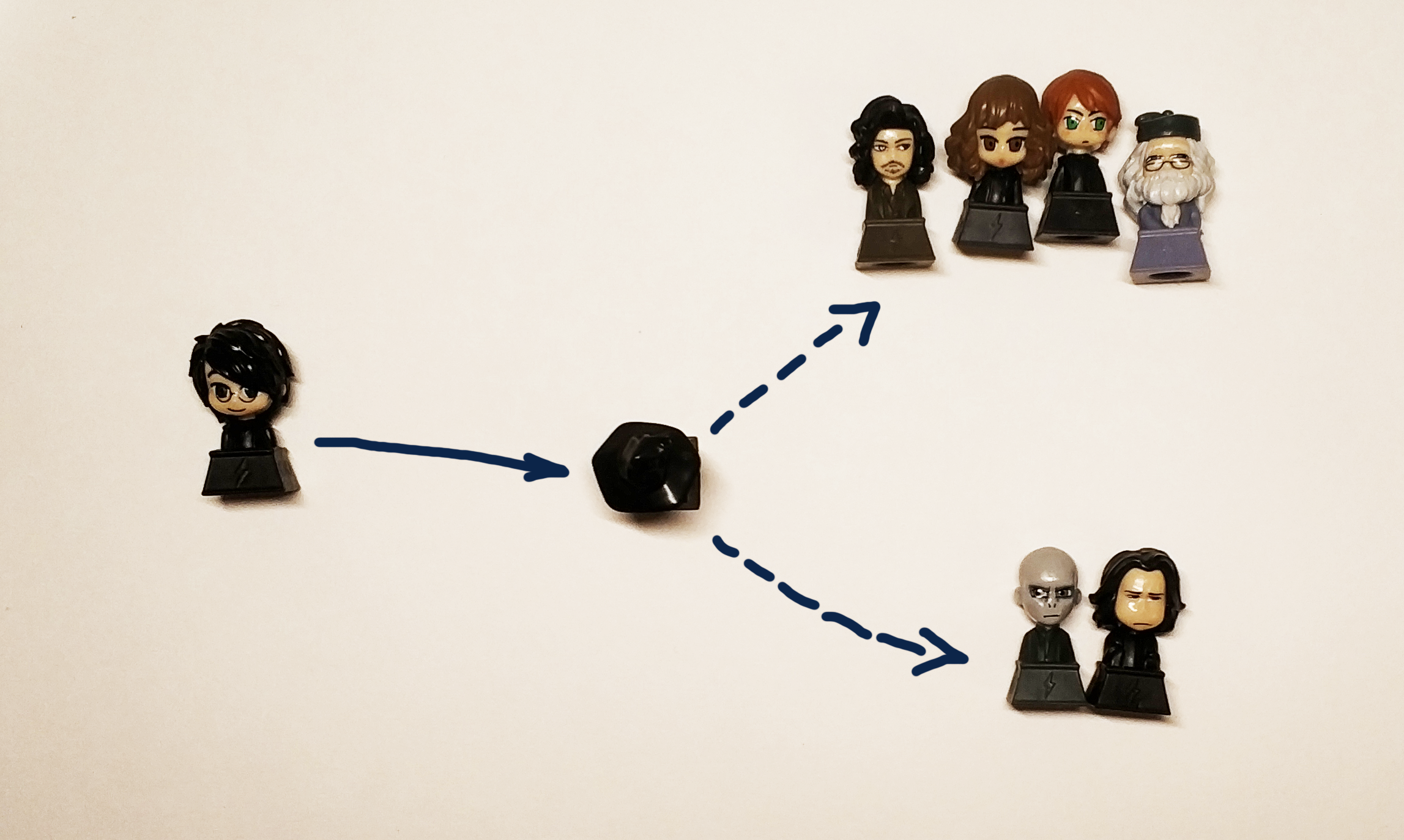
" " => [?] => Griffindor 

The original black hat distributed the young wizards to the faculties, depending on their character and personal qualities. Since the data on the character and personality of the task is not available to us, we will use the participant’s first and last name, remembering that in this case we must distribute the characters of the book to those departments that correspond to their native departments from the book. Yes, and the Potter lovers will definitely get upset if our solution distributes Harry to Puffendoi or Kogtevran (but it must send Harry and Slytherin to Harry with the same probability in order to convey the spirit of the book).

If we are talking about probabilities, then we formalize the problem in more rigorous mathematical terms. From the point of view of Data Science, we solve the problem of classification, namely, assigning an object (a string, in the form of a first and last name) of a certain class (in fact, it’s just a label, or a label, which can be a digit or 4 variables that have a yes / no value ). We understand that at least in the case of Harry it will be correct to give 2 answers: Gryffindor and Slytherin, so it’s better not to predict the particular department that the hat determines, but the probability that a person will be distributed to this department, therefore our decision will be kind of some function

Metrics and quality assessment

The task and goal are formulated, now we will think how to solve it , But that is not all. In order to proceed to the study, you need to enter the quality metrics. In other words - to determine how we will compare 2 different solutions among themselves.

Everything in life is good and simple - we intuitively understand that a spam detector must skip a minimum of spam to the inbox, and also skip a maximum of necessary letters and he certainly shouldn't send the necessary letters to spam.

In reality, it is becoming more complicated and confirming this a large number of articles that explain how and which metrics are used. The best practice is to understand this, but this is such a voluminous topic that we promise to write a separate post about it and make an open table so that everyone can play around and understand in practice how it differs.

The household “let's choose the best” for us will be the ROC AUC . This is exactly what we want from the metric in this case: the less false positives and the more accurate the actual prediction, the greater will be the ROC AUC.

In the ideal model, the ROC AUC is 1, in the ideal random model, which defines classes absolutely randomly - 0.5.

Algorithms

Our black box should take into account the distribution of the heroes of the books, take a different name and surname as input and output the result. To solve the classification problem, you can use different machine learning algorithms:

neural networks, factorization machines, linear regression or, for example, SVM.

Contrary to popular opinion, Data Science is not limited to neural networks alone, and to popularize this idea, in this article, neural networks are left as an exercise for the curious reader . Those who did not take a single course on data analysis (especially subjectively the best - from SLM), or simply read n news about machine learning or AI, which are now even published in the Amateur Fisherman magazines, probably met the names of general algorithms groups : bagging, boosting, support vector machine (SVM), linear regression. That is what we will use to solve our problem.

And to be more precise, we compare with each other:

• Linear regression
• Boosting (XGboost, LightGBM)
• Decisive trees (strictly speaking, this is the same boosting, but we will take out separately: Extra Trees)
• Bagging (Random Forest)
• SVM

The task of distributing each Hogwarts student to one of the faculties we can solve by defining the appropriate faculty, but strictly speaking this task is reduced to solving the problem of determining the belonging to each class separately. Therefore, within the framework of this article we set ourselves the goal of getting 4 models, one for each department.

Data

Finding the right dataset for learning, and more importantly - legal for use in the right goals - is one of the most difficult and time consuming tasks in Data Science. For our task, the data we take from wikia in the world of Harry Potter. For example on this link you can find all the characters who studied at the faculty of Gryffindor. It is important that the data in this case, we use for non-commercial purposes, so we do not violate the license of this site.

For those who think that Data Scientists are such cool guys, I will go to Data Scientists, let them teach me, we remind you that there is such a step as cleaning and preparing data. The downloaded data must be manually moderated in order to remove, for example, the “Seventh Prefect of Gryffindor” and semi-automatically remove the “Unknown girl from Gryffindor”. In real work, a proportionally large part of the task is always associated with the preparation, cleaning, and restoration of missing values ​​in a dataset.

A bit of ctrl + c & ctrl + v and at the output we get 4 text files containing the names of the characters in 2 languages: English and Russian.

We study the collected data (EDA, Exploratory Data Analysis)

To this stage we have 4 files containing the names of the students of the faculties, let's take a closer look:

 $ ls ../input griffindor.txt hufflpuff.txt ravenclaw.txt slitherin.txt 

Each file contains 1 first and last names (if any) of the student per line:

 $ wc -l ../input/*.txt 250 ../input/griffindor.txt 167 ../input/hufflpuff.txt 180 ../input/ravenclaw.txt 254 ../input/slitherin.txt 851 total 

The collected data is:

 $ cat ../input/griffindor.txt | head -3 && cat ../input/griffindor.txt | tail -3      Charlie Stainforth Melanie Stanmore Stewart 

Our whole idea is based on the assumption that there is something in the names and surnames that our black box (or black hat) can learn to distinguish.

The algorithm can feed the lines as is, but the result will not be good, because the basic models will not be able to understand for themselves what “Draco” differs from “Harry”, therefore, we will need to extract the signs from our names and surnames.

Data Preparation (Feature Engineering)

Signs (or features, from the English. Feature - property) - these are the distinctive properties of the object. The number of times a person has changed work over the past year, the number of fingers on his left hand, the size of a car’s engine, whether the car’s mileage exceeds 100,000 km or not. All sorts of classifications of signs have been invented by a very large number; there is not any single system in this regard, and there can be no, therefore we will give examples of what signs can be:

1. Rational number
2. Category (up to 12, 12-18 or 18+)
3. Binary value (Returned the first loan or not)
4. Date, color, share, etc.

The search (or formation) of features (in English by Feature Engineering ) is very often allocated to a separate stage of research or the work of a data analysis specialist. In fact, in the process itself, common sense, experience, and testing of hypotheses help. Guessing the right signs at once is a matter of a combination of a full hand, fundamental knowledge and luck. Sometimes there is shamanism in this, but the general approach is very simple: you need to do what comes to mind, and then check whether the solution was improved by adding a new attribute. For example, as a sign for our task, we can take the number of sizzles in the name.

In the first version (because the real Data Science study is like a masterpiece, it can never be completed) of our model we will use the following attributes for the first and last names:

1. 1 and the last letter of the word - vowel or consonant
2. The number of double vowels and consonants
3. Number of vowels, consonants, deaf, voiced
4. First Name, Last Name Length
5. ...

For this, we take this repository as a basis and add a class so that it can be used for Latin letters. This will give us the opportunity to determine how each letter sounds.

 >> from Phonetic import RussianLetter, EnglishLetter >> RussianLetter('').classify() {'consonant': True, 'deaf': False, 'hard': False, 'mark': False, 'paired': False, 'shock': False, 'soft': False, 'sonorus': True, 'vowel': False} >> EnglishLetter('d').classify() {'consonant': True, 'deaf': False, 'hard': True, 'mark': False, 'paired': False, 'shock': False, 'soft': False, 'sonorus': True, 'vowel': False} 

Now we can define simple functions for calculating statistics, for example:

 def starts_with_letter(word, letter_type='vowel'): """   ,    . :param word:  :param letter_type: 'vowel'  'consonant'.   . :return: Boolean """ if len(word) == 0: return False return Letter(word[0]).classify()[letter_type] def count_letter_type(word): """       . :param word:  :param debug:    :return: :obj:`dict` of :obj:`str` => :int:count """ count = { 'consonant': 0, 'deaf': 0, 'hard': 0, 'mark': 0, 'paired': 0, 'shock': 0, 'soft': 0, 'sonorus': 0, 'vowel': 0 } for letter in word: classes = Letter(letter).classify() for key in count.keys(): if classes[key]: count[key] += 1 return count 

With these functions, we can get the first signs:

 from feature_engineering import * >> print("  («»): ", len(""))   («»): 5 >> print(" («»)   : ", starts_with_letter('', 'vowel'))  («»)   : True >> print(" («»)   : ", starts_with_letter('', 'consonant'))  («»)   : True >> count_Harry = count_letter_type("") >> print ("     («»): ", count_Harry['paired'])      («»): 1 

Strictly speaking, using these functions we can get some vector representation of the string, that is, we get the mapping:

Now we can present our data in the form of a dataset, which can be input to the machine learning algorithm:

 >> from data_loaders import load_processed_data >> hogwarts_df = load_processed_data() >> hogwarts_df.head()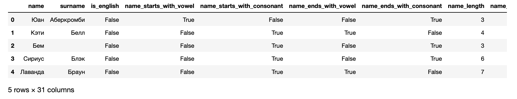 

As a result, we get the following signs for each student:

 >> hogwarts_df[hogwarts_df.columns].dtypes 

 name object surname object is_english bool name_starts_with_vowel bool name_starts_with_consonant bool name_ends_with_vowel bool name_ends_with_consonant bool name_length int64 name_vowels_count int64 name_double_vowels_count int64 name_consonant_count int64 name_double_consonant_count int64 name_paired_count int64 name_deaf_count int64 name_sonorus_count int64 surname_starts_with_vowel bool surname_starts_with_consonant bool surname_ends_with_vowel bool surname_ends_with_consonant bool surname_length int64 surname_vowels_count int64 surname_double_vowels_count int64 surname_consonant_count int64 surname_double_consonant_count int64 surname_paired_count int64 surname_deaf_count int64 surname_sonorus_count int64 is_griffindor int64 is_hufflpuff int64 is_ravenclaw int64 is_slitherin int64 dtype: object 

The last 4 columns are targeted - they contain information on which faculty the student is enrolled for.

Learning algorithms

In a nutshell, algorithms are trained the same way as people: they make mistakes and learn from them. In order to understand how badly they made a mistake, the algorithms use the error functions (loss functions, the English loss-function ).

As a rule, the learning process is very simple and it consists of several steps:

1. Make a prediction.
2. Rate the error.
3. Amend the model parameters.
4. Repeat 1-3 until the goal is reached, the process does not stop or the data runs out.

5. Rate the quality of the model.

   
   

   In practice, of course, everything is a little more complicated. For example, there is the phenomenon of retraining ( English overfitting) - the algorithm can literally remember which signs correspond to the answer and thus worsen the result for objects that are not similar to those for which it was trained. To avoid this, there are various techniques and hacks.

   
   

As mentioned above, we will solve 4 tasks: one for each faculty. Therefore, we prepare data for Slytherin:

 #  ,     - : >> data_full = hogwarts_df.drop( [ 'name', 'surname', 'is_griffindor', 'is_hufflpuff', 'is_ravenclaw' ], axis=1).copy() #    ,   : >> X_data = data_full.drop('is_slitherin', axis=1) #     ,   1    >> y = data_full.is_slitherin 

While learning, the algorithm constantly compares its results with real data, for this part of the dataset is allocated for validation. The rule of good tone is also considered to evaluate the result of the algorithm on individual data that the algorithm has never seen. Therefore, we now divide the sample in the proportion of 70/30 and train the first algorithm:

 from sklearn.cross_validation import train_test_split from sklearn.ensemble import RandomForestClassifier #      >> seed = 7 #    >> test_size = 0.3 >> X_train, X_test, y_train, y_test = train_test_split(X_data, y, test_size=test_size, random_state=seed) >> rfc = RandomForestClassifier() >> rfc_model = rfc.fit(X_train, y_train) 

Is done. Now, if you submit data to the input of this model, it will produce the result. This is fun, so first of all we will check if Harry’s model recognizes a Slytherin. To do this, we first prepare the functions in order to obtain the prediction of the algorithm:

 from data_loaders import parse_line_to_hogwarts_df import pandas as pd def get_single_student_features (name): """      :param name: string     :return: pd.DataFrame     """ featurized_person_df = parse_line_to_hogwarts_df(name) person_df = pd.DataFrame(featurized_person_df, columns=[ 'name', 'surname', 'is_english', 'name_starts_with_vowel', 'name_starts_with_consonant', 'name_ends_with_vowel', 'name_ends_with_consonant', 'name_length', 'name_vowels_count', 'name_double_vowels_count', 'name_consonant_count', 'name_double_consonant_count', 'name_paired_count', 'name_deaf_count', 'name_sonorus_count', 'surname_starts_with_vowel', 'surname_starts_with_consonant', 'surname_ends_with_vowel', 'surname_ends_with_consonant', 'surname_length', 'surname_vowels_count', 'surname_double_vowels_count', 'surname_consonant_count', 'surname_double_consonant_count', 'surname_paired_count', 'surname_deaf_count', 'surname_sonorus_count', ], index=[0] ) featurized_person = person_df.drop( ['name', 'surname'], axis = 1 ) return featurized_person def get_predictions_vector (model, person): """    :param model:   :param person: string   :return: list    """ encoded_person = get_single_student_features(person) return model.predict_proba(encoded_person)[0] 

And now we will set a small test dataset to consider the results of the algorithm.

 def score_testing_dataset (model): """      . :param model:   """ testing_dataset = [ " ", "Kirill Malev", " ", "Harry Potter", " ", " ","Severus Snape", " ", "Tom Riddle", " ", "Salazar Slytherin"] for name in testing_dataset: print ("{} — {}".format(name, get_predictions_vector(model, name)[1])) score_testing_dataset(rfc_model) 

   — 0.5 Kirill Malev — 0.5   — 0.0 Harry Potter — 0.0   — 0.75   — 0.9 Severus Snape — 0.5   — 0.2 Tom Riddle — 0.5   — 0.2 Salazar Slytherin — 0.3 

The results were dubious. Even the founder of the faculty would not get into his faculty, according to this model. Therefore, you need to evaluate the strict quality: look at the metrics that we asked at the beginning:

 from sklearn.metrics import accuracy_score, roc_auc_score, classification_report predictions = rfc_model.predict(X_test) print("Classification report: ") print(classification_report(y_test, predictions)) print("Accuracy for Random Forest Model: %.2f" % (accuracy_score(y_test, predictions) * 100)) print("ROC AUC from first Random Forest Model: %.2f" % (roc_auc_score(y_test, predictions))) 

 Classification report: precision recall f1-score support 0 0.66 0.88 0.75 168 1 0.38 0.15 0.21 89 avg / total 0.56 0.62 0.56 257 Accuracy for Random Forest Model: 62.26 ROC AUC from first Random Forest Model: 0.51 

It is not surprising that the results were so dubious - the ROC AUC of about 0.51 suggests that the model predicts slightly better than a coin toss.

Testing the results. Quality metrics

Above, using one example, we looked at how 1 algorithm that supports sklearn interfaces is trained. The rest are trained in exactly the same way, so we just have to train all the algorithms and choose the best in each case.

There is nothing difficult in this, for each algorithm we teach 1 with standard settings, and also we train a whole set, going through various options that affect the quality of the algorithm. This stage is called Model Tuning or Hyperparameter Optimization and its essence is very simple: choose the set of settings that gives the best result.

 from model_training import train_classifiers from data_loaders import load_processed_data import warnings warnings.filterwarnings('ignore') #   hogwarts_df = load_processed_data() #     data_full = hogwarts_df.drop( [ 'name', 'surname', 'is_griffindor', 'is_hufflpuff', 'is_ravenclaw' ], axis=1).copy() X_data = data_full.drop('is_slitherin', axis=1) y = data_full.is_slitherin #    slitherin_models = train_classifiers(data_full, X_data, y) score_testing_dataset(slitherin_models[5]) 

   — 0.09437856871661066 Kirill Malev — 0.20820536334902712   — 0.07550095601699099 Harry Potter — 0.07683794773639624   — 0.9414529336862744   — 0.9293671807790949 Severus Snape — 0.6576783576162999   — 0.18577792617672767 Tom Riddle — 0.8351835484058869   — 0.25930925139546795 Salazar Slytherin — 0.24008788903854789 

The numbers in this version look subjectively better than in the past, but are not good enough for an internal perfectionist. Therefore, we will go down to a level deeper and go back to the product meaning of our task: you need to predict the most probable faculty at which the hero will be assigned by the distribution hat. This means that you need to train models for each of the faculties.

 >> from model_training import train_all_models #      >> slitherin_models, griffindor_models, ravenclaw_models, hufflpuff_models = \ train_all_models() 

 SVM Default Report Accuracy for SVM Default: 73.93 ROC AUC for SVM Default: 0.53 Tuned SVM Report Accuracy for Tuned SVM: 72.37 ROC AUC for Tuned SVM: 0.50 KNN Default Report Accuracy for KNN Default: 70.04 ROC AUC for KNN Default: 0.58 Tuned KNN Report Accuracy for Tuned KNN: 69.65 ROC AUC for Tuned KNN: 0.58 XGBoost Default Report Accuracy for XGBoost Default: 70.43 ROC AUC for XGBoost Default: 0.54 Tuned XGBoost Report Accuracy for Tuned XGBoost: 68.09 ROC AUC for Tuned XGBoost: 0.56 Random Forest Default Report Accuracy for Random Forest Default: 73.93 ROC AUC for Random Forest Default: 0.62 Tuned Random Forest Report Accuracy for Tuned Random Forest: 74.32 ROC AUC for Tuned Random Forest: 0.54 Extra Trees Default Report Accuracy for Extra Trees Default: 69.26 ROC AUC for Extra Trees Default: 0.57 Tuned Extra Trees Report Accuracy for Tuned Extra Trees: 73.54 ROC AUC for Tuned Extra Trees: 0.55 LGBM Default Report Accuracy for LGBM Default: 70.82 ROC AUC for LGBM Default: 0.62 Tuned LGBM Report Accuracy for Tuned LGBM: 74.71 ROC AUC for Tuned LGBM: 0.53 RGF Default Report Accuracy for RGF Default: 70.43 ROC AUC for RGF Default: 0.58 Tuned RGF Report Accuracy for Tuned RGF: 71.60 ROC AUC for Tuned RGF: 0.60 FRGF Default Report Accuracy for FRGF Default: 68.87 ROC AUC for FRGF Default: 0.59 Tuned FRGF Report Accuracy for Tuned FRGF: 69.26 ROC AUC for Tuned FRGF: 0.59 SVM Default Report Accuracy for SVM Default: 70.43 ROC AUC for SVM Default: 0.50 Tuned SVM Report Accuracy for Tuned SVM: 71.60 ROC AUC for Tuned SVM: 0.50 KNN Default Report Accuracy for KNN Default: 63.04 ROC AUC for KNN Default: 0.49 Tuned KNN Report Accuracy for Tuned KNN: 65.76 ROC AUC for Tuned KNN: 0.50 XGBoost Default Report Accuracy for XGBoost Default: 69.65 ROC AUC for XGBoost Default: 0.54 Tuned XGBoost Report Accuracy for Tuned XGBoost: 68.09 ROC AUC for Tuned XGBoost: 0.50 Random Forest Default Report Accuracy for Random Forest Default: 66.15 ROC AUC for Random Forest Default: 0.51 Tuned Random Forest Report Accuracy for Tuned Random Forest: 70.43 ROC AUC for Tuned Random Forest: 0.50 Extra Trees Default Report Accuracy for Extra Trees Default: 64.20 ROC AUC for Extra Trees Default: 0.49 Tuned Extra Trees Report Accuracy for Tuned Extra Trees: 70.82 ROC AUC for Tuned Extra Trees: 0.51 LGBM Default Report Accuracy for LGBM Default: 67.70 ROC AUC for LGBM Default: 0.56 Tuned LGBM Report Accuracy for Tuned LGBM: 70.82 ROC AUC for Tuned LGBM: 0.50 RGF Default Report Accuracy for RGF Default: 66.54 ROC AUC for RGF Default: 0.52 Tuned RGF Report Accuracy for Tuned RGF: 65.76 ROC AUC for Tuned RGF: 0.53 FRGF Default Report Accuracy for FRGF Default: 65.76 ROC AUC for FRGF Default: 0.53 Tuned FRGF Report Accuracy for Tuned FRGF: 69.65 ROC AUC for Tuned FRGF: 0.52 SVM Default Report Accuracy for SVM Default: 74.32 ROC AUC for SVM Default: 0.50 Tuned SVM Report Accuracy for Tuned SVM: 74.71 ROC AUC for Tuned SVM: 0.51 KNN Default Report Accuracy for KNN Default: 69.26 ROC AUC for KNN Default: 0.48 Tuned KNN Report Accuracy for Tuned KNN: 73.15 ROC AUC for Tuned KNN: 0.49 XGBoost Default Report Accuracy for XGBoost Default: 72.76 ROC AUC for XGBoost Default: 0.49 Tuned XGBoost Report Accuracy for Tuned XGBoost: 74.32 ROC AUC for Tuned XGBoost: 0.50 Random Forest Default Report Accuracy for Random Forest Default: 73.93 ROC AUC for Random Forest Default: 0.52 Tuned Random Forest Report Accuracy for Tuned Random Forest: 74.32 ROC AUC for Tuned Random Forest: 0.50 Extra Trees Default Report Accuracy for Extra Trees Default: 73.93 ROC AUC for Extra Trees Default: 0.52 Tuned Extra Trees Report Accuracy for Tuned Extra Trees: 73.93 ROC AUC for Tuned Extra Trees: 0.50 LGBM Default Report Accuracy for LGBM Default: 73.54 ROC AUC for LGBM Default: 0.52 Tuned LGBM Report Accuracy for Tuned LGBM: 74.32 ROC AUC for Tuned LGBM: 0.50 RGF Default Report Accuracy for RGF Default: 73.54 ROC AUC for RGF Default: 0.51 Tuned RGF Report Accuracy for Tuned RGF: 73.93 ROC AUC for Tuned RGF: 0.50 FRGF Default Report Accuracy for FRGF Default: 73.93 ROC AUC for FRGF Default: 0.53 Tuned FRGF Report Accuracy for Tuned FRGF: 73.93 ROC AUC for Tuned FRGF: 0.50 SVM Default Report Accuracy for SVM Default: 80.54 ROC AUC for SVM Default: 0.50 Tuned SVM Report Accuracy for Tuned SVM: 80.93 ROC AUC for Tuned SVM: 0.52 KNN Default Report Accuracy for KNN Default: 78.60 ROC AUC for KNN Default: 0.50 Tuned KNN Report Accuracy for Tuned KNN: 80.16 ROC AUC for Tuned KNN: 0.51 XGBoost Default Report Accuracy for XGBoost Default: 80.54 ROC AUC for XGBoost Default: 0.50 Tuned XGBoost Report Accuracy for Tuned XGBoost: 77.04 ROC AUC for Tuned XGBoost: 0.52 Random Forest Default Report Accuracy for Random Forest Default: 77.43 ROC AUC for Random Forest Default: 0.49 Tuned Random Forest Report Accuracy for Tuned Random Forest: 80.54 ROC AUC for Tuned Random Forest: 0.50 Extra Trees Default Report Accuracy for Extra Trees Default: 76.26 ROC AUC for Extra Trees Default: 0.48 Tuned Extra Trees Report Accuracy for Tuned Extra Trees: 78.60 ROC AUC for Tuned Extra Trees: 0.50 LGBM Default Report Accuracy for LGBM Default: 75.49 ROC AUC for LGBM Default: 0.51 Tuned LGBM Report Accuracy for Tuned LGBM: 80.54 ROC AUC for Tuned LGBM: 0.50 RGF Default Report Accuracy for RGF Default: 78.99 ROC AUC for RGF Default: 0.52 Tuned RGF Report Accuracy for Tuned RGF: 75.88 ROC AUC for Tuned RGF: 0.55 FRGF Default Report Accuracy for FRGF Default: 76.65 ROC AUC for FRGF Default: 0.50 #   ,        

 from sklearn.linear_model import LogisticRegression clf = LogisticRegression(random_state=0, solver='lbfgs', multi_class='multinomial') hogwarts_df = load_processed_data_multi() #     data_full = hogwarts_df.drop( [ 'name', 'surname', ], axis=1).copy() X_data = data_full.drop('faculty', axis=1) y = data_full.faculty clf.fit(X_data, y) score_testing_dataset(clf) 

   — [0.3602361 0.16166944 0.16771712 0.31037733] Kirill Malev — [0.47473072 0.16051924 0.13511385 0.22963619]   — [0.38697926 0.19330242 0.17451052 0.2452078 ] Harry Potter — [0.40245098 0.16410043 0.16023278 0.27321581]   — [0.13197025 0.16438855 0.17739254 0.52624866]   — [0.17170203 0.1205678 0.14341742 0.56431275] Severus Snape — [0.15558044 0.21589378 0.17370406 0.45482172]   — [0.39301231 0.07397324 0.1212741 0.41174035] Tom Riddle — [0.26623969 0.14194379 0.1728505 0.41896601]   — [0.24843037 0.21632736 0.21532696 0.3199153 ] Salazar Slytherin — [0.09359144 0.26735897 0.2742305 0.36481909] 

 confusion_matrix(clf.predict(X_data), y) 

 array([[144, 68, 64, 78], [ 8, 9, 8, 6], [ 22, 18, 31, 20], [ 77, 73, 78, 151]]) 

 def get_predctions_vector (models, person): predictions = [get_predictions_vector (model, person)[1] for model in models] return { 'slitherin': predictions[0], 'griffindor': predictions[1], 'ravenclaw': predictions[2], 'hufflpuff': predictions[3] } def score_testing_dataset (models): testing_dataset = [ " ", "Kirill Malev", " ", "Harry Potter", " ", " ","Severus Snape", " ", "Tom Riddle", " ", "Salazar Slytherin"] data = [] for name in testing_dataset: predictions = get_predctions_vector(models, name) predictions['name'] = name data.append(predictions) scoring_df = pd.DataFrame(data, columns=['name', 'slitherin', 'griffindor', 'hufflpuff', 'ravenclaw']) return scoring_df # Data Science —    ,       top_models = [ slitherin_models[3], griffindor_models[3], ravenclaw_models[3], hufflpuff_models[3] ] score_testing_dataset(top_models) 

  name slitherin griffindor hufflpuff ravenclaw 0   0.349084 0.266909 0.110311 0.091045 1 Kirill Malev 0.289914 0.376122 0.384986 0.103056 2   0.338258 0.400841 0.016668 0.124825 3 Harry Potter 0.245377 0.357934 0.026287 0.154592 4   0.917423 0.126997 0.176640 0.096570 5   0.969693 0.106384 0.150146 0.082195 6 Severus Snape 0.663732 0.259189 0.290252 0.074148 7   0.268466 0.579401 0.007900 0.083195 8 Tom Riddle 0.639731 0.541184 0.084395 0.156245 9   0.653595 0.147506 0.172940 0.137134 10 Salazar Slytherin 0.647399 0.169964 0.095450 0.26126 

, . ROC AUC , 0.5. , :

• ;
• ;
• , ;
• , ;
• , , .

, , , , XGBoost CV , .

Important! , 70% . , 4 .

 from model_training import train_production_models from xgboost import XGBClassifier best_models = [] for i in range (0,4): best_models.append(XGBClassifier(base_score=0.5, booster='gbtree', colsample_bylevel=1, colsample_bytree=0.7, gamma=0, learning_rate=0.05, max_delta_step=0, max_depth=6, min_child_weight=11, missing=-999, n_estimators=1000, n_jobs=1, nthread=4, objective='binary:logistic', random_state=0, reg_alpha=0, reg_lambda=1, scale_pos_weight=1, seed=1337, silent=1, subsample=0.8)) slitherin_model, griffindor_model, ravenclaw_model, hufflpuff_model = \ train_production_models(best_models) top_models = slitherin_model, griffindor_model, ravenclaw_model, hufflpuff_model score_testing_dataset(top_models) 

 name slitherin griffindor hufflpuff ravenclaw 0   0.273713 0.372337 0.065923 0.279577 1 Kirill Malev 0.401603 0.761467 0.111068 0.023902 2   0.031540 0.616535 0.196342 0.217829 3 Harry Potter 0.183760 0.422733 0.119393 0.173184 4   0.945895 0.021788 0.209820 0.019449 5   0.950932 0.088979 0.084131 0.012575 6 Severus Snape 0.634035 0.088230 0.249871 0.036682 7   0.426440 0.431351 0.028444 0.083636 8 Tom Riddle 0.816804 0.136530 0.069564 0.035500 9   0.409634 0.213925 0.028631 0.252723 10 Salazar Slytherin 0.824590 0.067910 0.111147 0.085710 

, , .

, , . .

 import pickle pickle.dump(slitherin_model, open("../output/slitherin.xgbm", "wb")) pickle.dump(griffindor_model, open("../output/griffindor.xgbm", "wb")) pickle.dump(ravenclaw_model, open("../output/ravenclaw.xgbm", "wb")) pickle.dump(hufflpuff_model, open("../output/hufflpuff.xgbm", "wb")) 

, . , , , .

, , . , . , Data Scientist — -.

:

• ;
• json- json;
• .

, docker-, python-. , flask.

 from __future__ import print_function # In python 2.7 import os import subprocess import json import re from flask import Flask, request, jsonify from inspect import getmembers, ismethod import numpy as npb import pandas as pd import math import os import pickle import xgboost as xgb import sys from letter import Letter from talking_hat import * from sklearn.ensemble import RandomForestClassifier import warnings def prod_predict_classes_for_name (full_name): featurized_person = parse_line_to_hogwarts_df(full_name) person_df = pd.DataFrame(featurized_person, columns=[ 'name', 'surname', 'is_english', 'name_starts_with_vowel', 'name_starts_with_consonant', 'name_ends_with_vowel', 'name_ends_with_consonant', 'name_length', 'name_vowels_count', 'name_double_vowels_count', 'name_consonant_count', 'name_double_consonant_count', 'name_paired_count', 'name_deaf_count', 'name_sonorus_count', 'surname_starts_with_vowel', 'surname_starts_with_consonant', 'surname_ends_with_vowel', 'surname_ends_with_consonant', 'surname_length', 'surname_vowels_count', 'surname_double_vowels_count', 'surname_consonant_count', 'surname_double_consonant_count', 'surname_paired_count', 'surname_deaf_count', 'surname_sonorus_count', ], index=[0] ) slitherin_model = pickle.load(open("models/slitherin.xgbm", "rb")) griffindor_model = pickle.load(open("models/griffindor.xgbm", "rb")) ravenclaw_model = pickle.load(open("models/ravenclaw.xgbm", "rb")) hufflpuff_model = pickle.load(open("models/hufflpuff.xgbm", "rb")) predictions = get_predctions_vector([ slitherin_model, griffindor_model, ravenclaw_model, hufflpuff_model ], person_df.drop(['name', 'surname'], axis=1)) return { 'slitherin': float(predictions[0][1]), 'griffindor': float(predictions[1][1]), 'ravenclaw': float(predictions[2][1]), 'hufflpuff': float(predictions[3][1]) } def predict(params): fullname = params['fullname'] print(params) return prod_predict_classes_for_name(fullname) def create_app(): app = Flask(__name__) functions_list = [predict] @app.route('/<func_name>', methods=['POST']) def api_root(func_name): for function in functions_list: if function.__name__ == func_name: try: json_req_data = request.get_json() if json_req_data: res = function(json_req_data) else: return jsonify({"error": "error in receiving the json input"}) except Exception as e: data = { "error": "error while running the function" } if hasattr(e, 'message'): data['message'] = e.message elif len(e.args) >= 1: data['message'] = e.args[0] return jsonify(data) return jsonify({"success": True, "result": res}) output_string = 'function: %s not found' % func_name return jsonify({"error": output_string}) return app if __name__ == '__main__': app = create_app() app.run(host='0.0.0.0') 

Dockerfile:

 FROM datmo/python-base:cpu-py35 #  python3-wheel,        RUN apt-get update; apt-get install -y python3-pip python3-numpy python3-scipy python3-wheel ADD requirements.txt / RUN pip3 install -r /requirements.txt RUN mkdir /code;mkdir /code/models COPY ./python_api.py ./talking_hat.py ./letter.py ./request.py /code/ COPY ./models/* /code/models/ WORKDIR /code CMD python3 /code/python_api.py 

:

 docker build -t talking_hat . && docker rm talking_hat && docker run --name talking_hat -p 5000:5000 talking_hat 

— . , Apache Benchmark . , . — .

 $ ab -p data.json -T application/json -c 50 -n 10000 http://0.0.0.0:5000/predict 

 This is ApacheBench, Version 2.3 <$Revision: 1807734 $> Copyright 1996 Adam Twiss, Zeus Technology Ltd, http://www.zeustech.net/ Licensed to The Apache Software Foundation, http://www.apache.org/ Benchmarking 0.0.0.0 (be patient) Completed 1000 requests Completed 2000 requests Completed 3000 requests Completed 4000 requests Completed 5000 requests Completed 6000 requests Completed 7000 requests Completed 8000 requests Completed 9000 requests Completed 10000 requests Finished 10000 requests Server Software: Werkzeug/0.14.1 Server Hostname: 0.0.0.0 Server Port: 5000 Document Path: /predict Document Length: 141 bytes Concurrency Level: 50 Time taken for tests: 238.552 seconds Complete requests: 10000 Failed requests: 0 Total transferred: 2880000 bytes Total body sent: 1800000 HTML transferred: 1410000 bytes Requests per second: 41.92 [#/sec] (mean) Time per request: 1192.758 [ms] (mean) Time per request: 23.855 [ms] (mean, across all concurrent requests) Transfer rate: 11.79 [Kbytes/sec] received 7.37 kb/s sent 19.16 kb/s total Connection Times (ms) min mean[+/-sd] median max Connect: 0 0 0.1 0 3 Processing: 199 1191 352.5 1128 3352 Waiting: 198 1190 352.5 1127 3351 Total: 202 1191 352.5 1128 3352 Percentage of the requests served within a certain time (ms) 50% 1128 66% 1277 75% 1378 80% 1451 90% 1668 95% 1860 98% 2096 99% 2260 100% 3352 (longest request) 

, :

 def prod_predict_classes_for_name (full_name): <...> predictions = get_predctions_vector([ app.slitherin_model, app.griffindor_model, app.ravenclaw_model, app.hufflpuff_model ], person_df.drop(['name', 'surname'], axis=1)) return { 'slitherin': float(predictions[0][1]), 'griffindor': float(predictions[1][1]), 'ravenclaw': float(predictions[2][1]), 'hufflpuff': float(predictions[3][1]) } def create_app(): <...> with app.app_context(): app.slitherin_model = pickle.load(open("models/slitherin.xgbm", "rb")) app.griffindor_model = pickle.load(open("models/griffindor.xgbm", "rb")) app.ravenclaw_model = pickle.load(open("models/ravenclaw.xgbm", "rb")) app.hufflpuff_model = pickle.load(open("models/hufflpuff.xgbm", "rb")) return app 

:

 $ docker build -t talking_hat . && docker rm talking_hat && docker run --name talking_hat -p 5000:5000 talking_hat $ ab -p data.json -T application/json -c 50 -n 10000 http://0.0.0.0:5000/predict 

 This is ApacheBench, Version 2.3 <$Revision: 1807734 $> Copyright 1996 Adam Twiss, Zeus Technology Ltd, http://www.zeustech.net/ Licensed to The Apache Software Foundation, http://www.apache.org/ Benchmarking 0.0.0.0 (be patient) Completed 1000 requests Completed 2000 requests Completed 3000 requests Completed 4000 requests Completed 5000 requests Completed 6000 requests Completed 7000 requests Completed 8000 requests Completed 9000 requests Completed 10000 requests Finished 10000 requests Server Software: Werkzeug/0.14.1 Server Hostname: 0.0.0.0 Server Port: 5000 Document Path: /predict Document Length: 141 bytes Concurrency Level: 50 Time taken for tests: 219.812 seconds Complete requests: 10000 Failed requests: 3 (Connect: 0, Receive: 0, Length: 3, Exceptions: 0) Total transferred: 2879997 bytes Total body sent: 1800000 HTML transferred: 1409997 bytes Requests per second: 45.49 [#/sec] (mean) Time per request: 1099.062 [ms] (mean) Time per request: 21.981 [ms] (mean, across all concurrent requests) Transfer rate: 12.79 [Kbytes/sec] received 8.00 kb/s sent 20.79 kb/s total Connection Times (ms) min mean[+/-sd] median max Connect: 0 0 0.1 0 2 Processing: 235 1098 335.2 1035 3464 Waiting: 235 1097 335.2 1034 3462 Total: 238 1098 335.2 1035 3464 Percentage of the requests served within a certain time (ms) 50% 1035 66% 1176 75% 1278 80% 1349 90% 1541 95% 1736 98% 1967 99% 2141 100% 3464 (longest request) 

Is done. . , .

Conclusion

, . - .

, :

• feature engineering- ( ), , Soundex .
• PyTorch . , , .
• flask Quart , , .
• - -, .

, , . , !

This article would not have been published without the Open Data Science community, which brings together a large number of Russian-speaking data analysis specialists.