There is such a popular class of tasks in which it is required to conduct a sufficiently deep analysis of the entire volume of work chains recorded by some information system (IS). Document management, desktops, bugtrackers, e-journals, inventory accounting, etc. can be used as IPs. The nuances are manifested in data models, APIs, data volumes, and other aspects, but the principles for solving such problems are about the same. And the rake, which can be stepped on, is also very similar.

To solve this class of problems, R fits perfectly. But, in order not to let go of disappointed hands, that R may be good, but oh, very slow, it is important to pay attention to the performance of the chosen data processing methods.

It is a continuation of previous publications .

Usually, a head-on approach is not the most effective. 99% of the tasks associated with the analysis and processing of data begin with their import. In this brief essay, we will look at the problems that arise at the basic stage of importing data with data in json format, using the example of a typical “in-depth” analysis of Jira installation data as an example. json supports a complex object model, in contrast to csv , so its parsing in the case of complex structures can become very difficult and long.

Formulation of the problem

Given:

• jira is implemented and used in the software development process as a task management system and bugtracker.
• There is no direct access to the jira database, the interaction is carried out through the REST API (galvanic isolation).
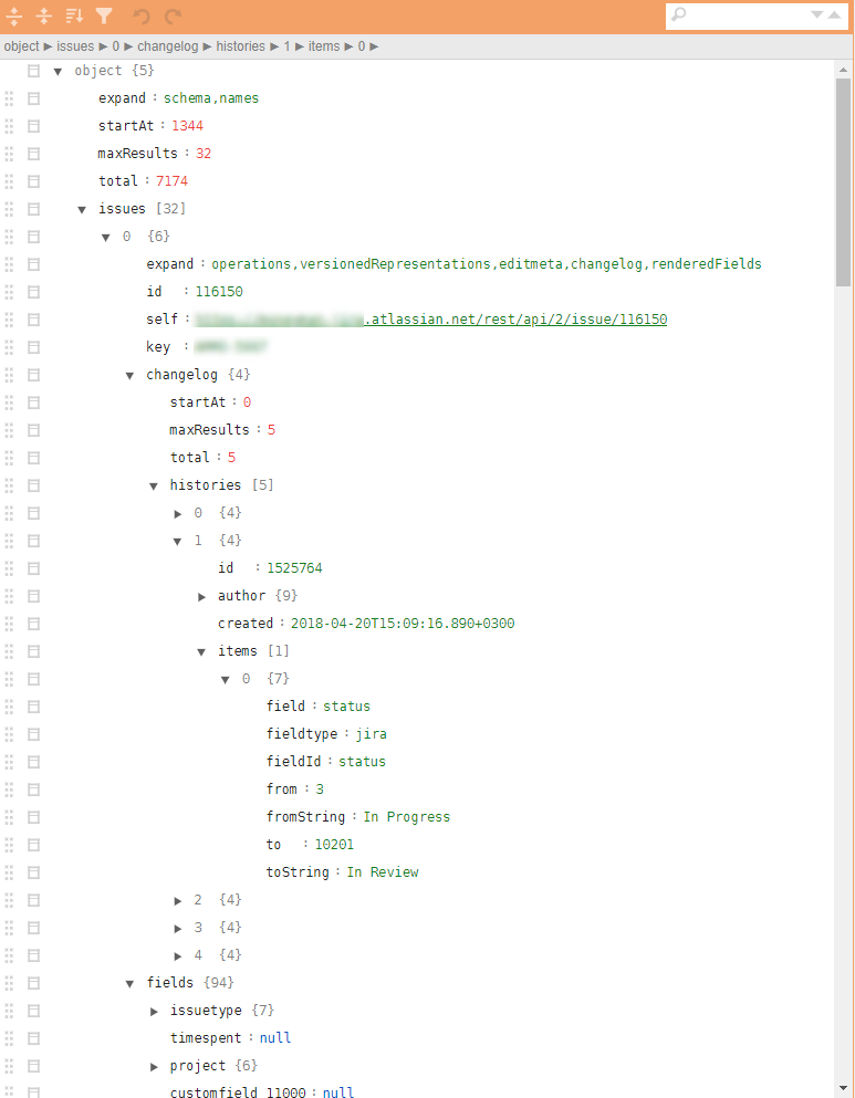
• Pickup json files have a very complex tree structure with nested tuples required to upload the entire history of actions. To calculate the same metrics, a relatively small number of parameters are needed, scattered across different levels of the hierarchy.

An example of a regular jira json in the figure.

Required:

• Based on jira data, it is necessary to find the bottlenecks and points of possible growth in the efficiency of development processes and improve the quality of the resulting product based on the analysis of all recorded activities.

Decision

Theoretically, in R there are several different packages for downloading json and converting them into data.frame . The most convenient is the jsonlite package. However, the direct transformation of the json hierarchy in data.frame difficult due to the multi-level nesting and strong parametrization of the record structure. Linking specific parameters related, for example, to the history of actions, may require various add. checks and cycles. Those. The task can be solved, but for a json file with a size of 32 tasks (includes all artifacts and the entire history of tasks), such non-linear analysis using jsonlite and tidyverse takes ~ 10 seconds on an average performance laptop.

By themselves, 10 seconds is a bit. But just until the moment these files become too many. Estimation of the sample parsing and loading of such a "direct" method ~ 4000 files (~ 4 GB) gave 8-9 hours of work.

Such a large number of files appeared for a reason. First, jira has a time limit on the REST session, it’s impossible to pull out all the bulk. Secondly, being embedded in the production contour, the daily upload of data on the updated tasks is expected. Thirdly, and this will be mentioned later, the task is very good for linear scaling and you need to think about parallelization from the very first step.

Even 10–15 iterations at the stage of data analysis, identifying the required minimum set of parameters, detecting exceptional or erroneous situations, and developing post-processing algorithms result in costs of 2–3 weeks (only counting time).
Naturally, such a “performance” is not suitable for operational analytics embedded in the productive contour, and is very ineffective at the stage of the initial data analysis and development of the prototype.

Skipping all intermediate details, I immediately turn to the answer. We recall Donald Knuth, roll up our sleeves and begin to engage in microbenchmarking of all key operations mercilessly cutting off everything that is possible.

The resulting solution is reduced to the following 10 lines (this is a common skeleton, without a subsequent non-functional body kit):

 library(tidyverse) library(jsonlite) library(readtext) fnames <- fs::dir_ls(here::here("input_data"), glob = "*.txt") ff <- function(fname){ json_vec <- readtext(fname, text_field = "texts", encoding = "UTF-8") %>% .$text %>% jqr::jq('[. | {issues: .issues}[] | .[]', '{id: .id, key: .key, created: .fields.created, type: .fields.issuetype.name, summary: .fields.summary, descr: .fields.description}]') jsonlite::fromJSON(json_vec, flatten = TRUE) } tictoc::tic("Loading with jqr-jsonlite single-threaded technique") issues_df <- fnames %>% purrr::map(ff) %>% data.table::rbindlist(use.names = FALSE) tictoc::toc() system.time({fst::write_fst(issues_df, here::here("data", "issues.fst"))}) 

What is interesting here?

1. To speed up the boot process, it is good to use specialized profiled packages, such as readtext .
2. The use of the stream parser jq allows jq to translate all the hooking of the necessary attributes into a functional language, drop it to the CPP level and minimize manual manipulation of nested lists or lists in the data.frame .
3. A very promising bench package for microbench marks appeared. It allows you to study not only the execution time of operations, but also memory manipulations. It's no secret that you can lose a lot on copying data in memory.
4. For large amounts of data and simple processing, it is often necessary in the final decision to abandon the tidyverse and translate labor-intensive parts to data.table , in particular, it is here that the tables are merged by means of data.table . As well as all the transformations at the post-processing stage (which are included in the cycle using the ff function are also made by data.table with the approach of changing data by reference, or by packages built using Rcpp , for example, anytime package for working with dates and time.
5. The fst package is very good for resetting data to a file and subsequent reading. In particular, it only takes a fraction of a second to save all analytics of jira history for 4 years, and the data is saved as data types R, which is good for later reuse.

During the solution, an approach using the rjson package was rjson . The jsonlite::fromJSON about 2 times slower than rjson = rjson::fromJSON(json_vec) , but we had to leave it exactly, because NULL values ​​are in the data, and at the stage of converting NULL to NA in the lists issued by rjson we lose advantage, and the code is heavier.

Conclusion

1. Similar refactoring led to a change in the processing time of all json files in single-threaded mode on the same laptop from 8-9 hours to 10 minutes.
2. Adding task parallelization by means of foreach practically did not make the code (+ 5 lines) but reduced the execution time to 5 minutes.
3. Transferring the solution to a weak linux server (only 4 cores), but running on an SSD in multi-threaded mode reduced the execution time to 40 seconds.
4. The publication on the productive contour (20 cores, 3 GHz, SSD) reduced the execution time to 6-8 seconds, which is more than acceptable for operational analytics tasks.

Total, staying within the framework of the R platform, we managed to achieve a simple refactoring of the code by reducing the execution time from ~ 9 hours to ~ 9 seconds.

Solutions on R can be quite fast. If something goes wrong with you, try to look at it from a different angle and using fresh techniques.

Previous publication - "Analytical Plan for Manager . "