Julia and the movement of a charged particle in an electromagnetic field

We fix the skills of solving and visualizing differential equations on the example of one of the most common evolutionary equations, recall the good old Scilab and try to understand whether we need it ... Under the cut of the picture (kilobyte per seven hundred)
julia>] (v1.0) pkg>update # (v1.0) pkg> status Status `C:\Users\\.julia\environments\v1.0\Project.toml` [537997a7] AbstractPlotting v0.9.0 [ad839575] Blink v0.8.1 [159f3aea] Cairo v0.5.6 [5ae59095] Colors v0.9.5 [8f4d0f93] Conda v1.1.1 [0c46a032] DifferentialEquations v5.3.1 [a1bb12fb] Electron v0.3.0 [5789e2e9] FileIO v1.0.2 [5752ebe1] GMT v0.5.0 [28b8d3ca] GR v0.35.0 [c91e804a] Gadfly v1.0.0+ #master (https://github.com/GiovineItalia/Gadfly.jl.git) [4c0ca9eb] Gtk v0.16.4 [a1b4810d] Hexagons v0.2.0 [7073ff75] IJulia v1.14.1+ [`C:\Users\\.julia\dev\IJulia`] [6218d12a] ImageMagick v0.7.1 [c601a237] Interact v0.9.0 [b964fa9f] LaTeXStrings v1.0.3 [ee78f7c6] Makie v0.9.0+ #master (https://github.com/JuliaPlots/Makie.jl.git) [7269a6da] MeshIO v0.3.1 [47be7bcc] ORCA v0.2.0 [58dd65bb] Plotly v0.2.0 [f0f68f2c] PlotlyJS v0.12.0+ #master (https://github.com/sglyon/PlotlyJS.jl.git) [91a5bcdd] Plots v0.21.0 [438e738f] PyCall v1.18.5 [d330b81b] PyPlot v2.6.3 [c4c386cf] Rsvg v0.2.2 [60ddc479] StatPlots v0.8.1 [b8865327] UnicodePlots v0.3.1 [0f1e0344] WebIO v0.4.2 [c2297ded] ZMQ v1.0.0 Let's go through the previous guides
and proceed to the formulation of the problem
Motion of charged particles in the electromagnetic field
On a charged particle with a charge q moving in EMF with speed u Lorentz force acts: vecFL=q left( vecE+ left[ vecu times vecB right] right) . This formula is valid for a number of simplifications. Neglecting the corrections to the theory of relativity, we assume that the particle mass is constant, so that the equation of motion has the form: fracddt(m vecu)=q left( vecE+ left[ vecu times vecB right] right)
We direct the Y axis along the electric field, the Z axis along the magnetic field, and assume for simplicity that the initial velocity of the particle lies in the XY plane. In this case, the entire trajectory of the particle will also lie in this plane. The equations of motion will take the form:
\ left \ {\ begin {matrix} m \ ddot {x} = qB \ dot {y} \\ m \ ddot {y} = qE-qB \ dot {x} \ end {matrix} \ right.
Nondimensional: x∗= fracx lambda,y∗= fracy lambda, tau= fracct lambda,B∗= fracBmcq lambda,E∗= fracEmc2q lambda . Asterisks denote dimensional values, and lambda - the characteristic size of the considered physical system. We obtain the dimensionless system of equations of motion of a charged particle in a magnetic field:
\ left \ {\ begin {matrix} \ frac {d ^ 2x} {d \ tau ^ 2} = B \ frac {dy} {d \ tau} \\ \ frac {d ^ 2y} {d \ tau ^ 2} = EB \ frac {dx} {d \ tau} \ end {matrix} \ right.
Lower the order:
\ left \ {\ begin {matrix} \ frac {dx} {d \ tau} = U_x \\ \ frac {dy} {d \ tau} = U_y \\ \ frac {dU_x} {d \ tau} = BU_y \\ \ frac {dU_y} {d \ tau} = E-BU_x \ end {matrix} \ right.
As the initial configuration of the model, choose: B=2 Tl E=5 cdot104 V / m v0=7 cdot104 m / s For a numerical solution, we use the DifferentialEquations package:
using DifferentialEquations, Plots pyplot() M = 9.11e-31 # kg q = 1.6e-19 # C C = 3e8 # m/s λ = 1e-3 # m function modelsolver(Bo = 2., Eo = 5e4, vel = 7e4) B = Bo*q*λ / (M*C) E = Eo*q*λ / (M*C*C) vel /= C A = [0. 0. 1. 0.; 0. 0. 0. 1.; 0. 0. 0. B; 0. 0. -B 0.] syst(u,p,t) = A * u + [0.; 0.; 0.; E] # ODE system u0 = [0.0; 0.0; vel; 0.0] # start cond-ns tspan = (0.0, 6pi) # time period prob = ODEProblem(syst, u0, tspan) # problem to solve sol = solve(prob, Euler(), dt = 1e-4, save_idxs = [1, 2], timeseries_steps = 1000) end Solut = modelsolver() plot(Solut) 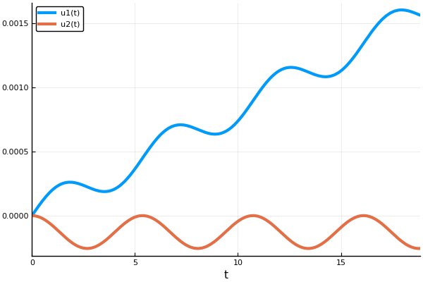
Here the Euler method is used, for which the number of steps is given. Also, not all the solution of the system is stored in the answer matrix, but only the 1 and 2 indices, that is, the X and Y coordinates (we do not need speed).
X = [Solut.u[i][1] for i in eachindex(Solut.u)] Y = [Solut.u[i][2] for i in eachindex(Solut.u)] plot(X, Y, xaxis=("X"), background_color=RGB(0.1, 0.1, 0.1)) title!(" ") yaxis!("Y") savefig("XY1.png")# 
Check the result. Let's introduce instead of x a new variable tildex=x−ut . Thus, a transition to a new coordinate system is carried out, moving relative to the initial one at a speed u in the direction of the X axis:
\ left \ {\ begin {matrix} \ ddot {\ tilde {x}} = qB \ dot {y} / m \\ \ ddot {y} = qE / m-qB \ dot {x} / m -qBu / m \ end {matrix} \ right.
If you choose u=E/B and mark omega=qB/m , the system will be simplified:
\ left \ {\ begin {matrix} \ ddot {\ tilde {x}} = \ omega \ dot {y} \\ \ ddot {y} = - \ omega \ dot {\ tilde {x}} \ end { matrix} \ right.
The electric field has disappeared from the last equations, and they represent the equations of motion of a particle under the action of a uniform magnetic field. Thus, the particle in the new coordinate system (x, y) should move in a circle. Since this new coordinate system itself moves relative to the original one at a speed u=E/B , then the resulting motion of the particle will consist of a uniform motion along the X axis and rotation around the circle in the XY plane. As is known, the trajectory arising from the addition of such two movements, in the general case, is a trochoid . In particular, if the initial velocity is zero, the simplest case of such a motion is realized - along the cycloid .
Let us make sure that the drift speed is really equal to E / B. For this:
- subtract the response matrix by replacing the first element (maximum) with the obviously lower value
- find the number of the maximum element in the second column of the matrix of answers, which is deposited on the ordinate
- calculate the dimensionless drift velocity by dividing the maximum abscissa value by the corresponding time value
Y[1] = -0.1 numax = argmax( Y ) X[numax] / Solut.t[numax] Out: 8.334546850446588e-5
B = 2*q*λ / (M*C) E = 5e4*q*λ / (M*C*C) E/B Out: 8.333333333333332e-5
Up to the seventh order!
For convenience, we will define a function that takes the parameters of the model and the signature of the graphic, which will also serve as the name of the png file created in the project folder (works in Juno / Atom and Jupyter). Unlike Gadfly , where graphs were created in layers , and then output by the plot () function, in Plots, in order to create different graphs in one frame, the first one is created by the plot () function, and subsequent ones are added using plot! () . The names of functions that change received objects in Julia are usually terminated with an exclamation mark.
function plotter(ttle = "qwerty", Bo = 2, Eo = 4e4, vel = 7e4) Ans = modelsolver(Bo, Eo, vel) X = [Ans.u[i][1] for i in eachindex(Ans.u)] Y = [Ans.u[i][2] for i in eachindex(Ans.u)] plot!(X, Y) p = title!(ttle) savefig( p, ttle * ".png" ) end At zero initial speed, as expected, we obtain a cycloid :
plot() plotter("Zero start velocity", 2, 4e4, 7e4) 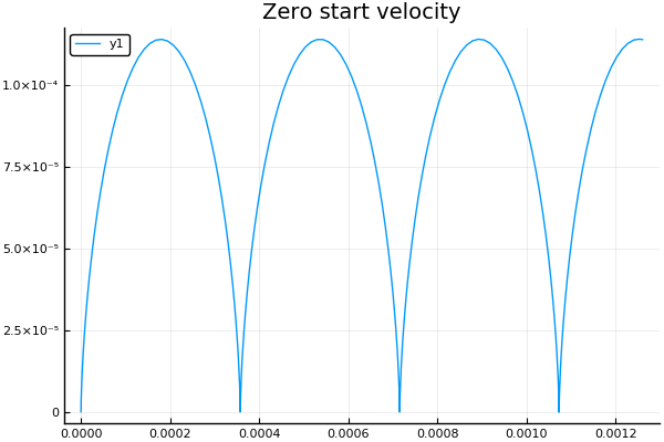
We obtain the trajectory of the particle when the induction is zeroed, the intensity and when the sign of the charge changes. Let me remind you that the dot means alternately performing the function with all the elements of the array
plot() plotter.("B ", 0, [3e4 4e4 5e4 6e4] ) 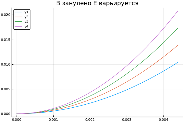
plot() plotter.("E B ", [1 2 3 4], 0 ) 
q = -1.6e-19 # C plot() plotter.(" ") 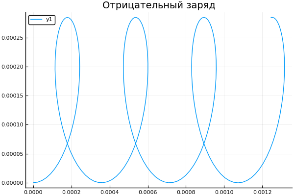
plot() plotter.(" ", 2, 5e4, [2e4 4e4 6e4 8e4] ) 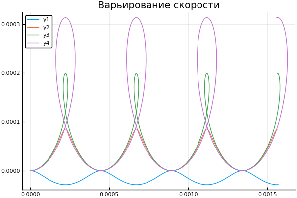
A bit about Scilab
On Habré there is already enough information about Sylab, for example, 1 , 2 , and here about Octave, therefore, we limit ourselves to links to Wikipedia and to the home page .
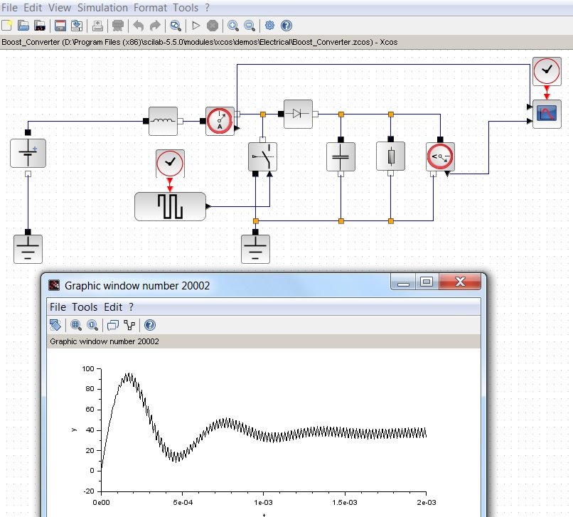
From myself I will add, about the presence of a convenient interface creation with checkboxes, buttons and graph output, and a rather interesting Xcos visual modeling tool. The latter can be used, for example, to simulate a signal in electrical engineering:

And here is a very convenient guide: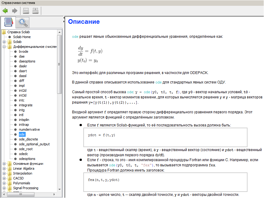
Actually, our task can be solved in Scilab:
clear function du = syst(t, u, A, E) du = A * u + [0; 0; 0; E] // ODE system end function [tspan, U] = modelsolver(Bo, Eo, vel) B = Bo*q*λ / (M*C) E = Eo*q*λ / (M*C*C) vel = vel / C u0 = [0; 0; vel; 0] // start cond-ns t0 = 0.0 tspan = t0:0.1:6*%pi // time period A = [0 0 1 0; 0 0 0 1; 0 0 0 B; 0 0 -B 0] U = ode("rk", u0, t0, tspan, list(syst, A, E) ) end M = 9.11e-31 // kg q = 1.6e-19 // C C = 3e8 // m/s λ = 1e-3 // m [cron, Ans1] = modelsolver( 2, 5e4, 7e4 ) plot(cron, Ans1 ) xtitle (" ","t","x, y, dx/dt, dy/dt"); legend ("x", "y", "Ux", "Uy"); scf(1)// plot(Ans1(1, :), Ans1(2, :) ) xtitle (" ","x","y"); xs2png(0,'graf1');// xs2jpg(1,'graf2');// , - 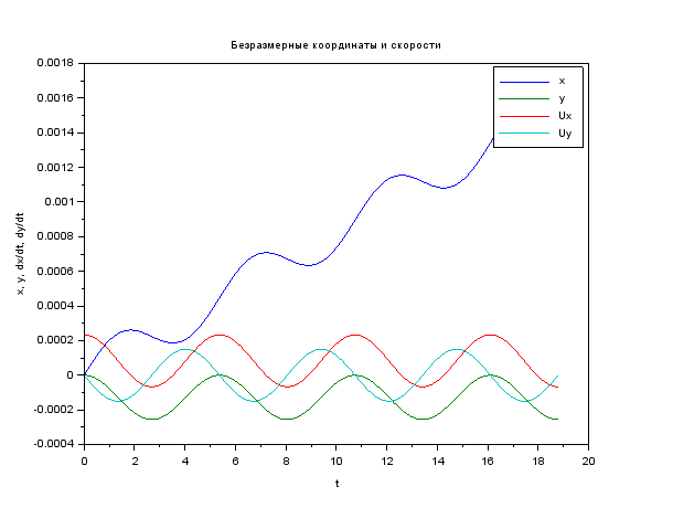

Here is the function information for solving ode diffs . In principle, the question arises
And why do we need Julia?
... if so there are such wonderful things as Scilab, Octave and Numpy, Scipy?
About the last two I will not say - did not try. And in general, the question is difficult, so let's estimate it:
Scilab
On a hard drive, it will take a little more than 500 MB, it starts up quickly and immediately both the differential reading, the graphics and everything else are available. Good for beginners: an excellent guide (mostly localized), there are many books in Russian. About internal errors have already been said here and here , and since the product is very niche, the community is sluggish, and the additional modules are very scarce.
Julia
With the addition of packages (especially of any pitonscale a la Jupyter and Mathplotlib) it grows from 376 MB to quite six more gigabytes. She also does not spare the operative: at the start of 132 MB, and after filling in the schedules in Jupiter, it will calmly reach 1 GB. If you work in Juno , then everything is almost like in Scilab : you can execute the code immediately in the interpreter, you can print in the built-in notepad and save as a file, there is a variable browser, command log and online help. Personally, I am indignant at the absence of clear () , that is, I launched the code, then began to correct and rename there, and the old variables remained (there is no variable browser in Jupiter).
But all this is not critical. Scilab fits perfectly on the first couple, making a lab, curving or counting something intermediate is a very useful tool. Although here, too, there is support for parallel computing and calling of sishnyh / Fortran functions, for which purpose it cannot be used seriously. Large arrays plunge it into horror, to set multidimensional, you have to do all sorts of obscurantism , and calculations beyond the framework of classical problems may well drop everything along with the operating system.
And after all these pains and disappointments, you can safely switch to Julia , in order to get more here. We will continue to learn, the benefit of the community is very responsive, problems get shaken quickly, and Julia has many interesting features that will make the learning process a fascinating journey!
')
Source: https://habr.com/ru/post/429790/
All Articles