Learn OpenGL. Lesson 6.4 - IBL. Mirror irradiance

In the previous lesson, we prepared our PBR model to work together with the IBL method — for this we needed to prepare in advance an irradiance map that describes the diffuse part of the indirect illumination. In this lesson we will pay attention to the second part of the expression of reflectivity - the mirror:

$$

$$L_o (p, \ omega_o) = \ int \ limits _ {\ Omega} (k_d \ frac {c} {\ pi} + k_s \ frac {DFG} {4 (\ omega_o \ cdot n) (\ omega_i \ cdot n )}) L_i (p, \ omega_i) n \ cdot \ omega_i d \ omega_i$$

It can be noted that the Cook’s-Torrens mirror component (the subexpression with the multiplier $$$k_s$ ) is not constant and depends on the direction of the incident light, as well as on the direction of observation. The solution of this integral for all possible directions of incidence of light, together with all possible directions of observation in real time, is simply not feasible. Therefore, Epic Games researchers have proposed an approach called split sum approximation , which allows partial data to be prepared for the mirror component in advance, subject to certain conditions.

In this approach, the mirror component of the expression of reflectivity is divided into two parts, which can be pre-convolved separately, and then combined into a PBR shader, to be used as a source of indirect mirror radiation. As with the formation of an irradiance map, the convolution process accepts an HDR environment map at its entrance.

To understand the method of approximation by a separate sum, look again at the expression of reflectivity, leaving only the subexpression for the mirror component in it (the diffuse part was considered separately in the previous lesson ):

$$

$$L_o (p, \ omega_o) = \ int \ limits _ {\ Omega} (k_s \ frac {DFG} {4 (\ omega_o \ cdot n) (\ omega_i \ cdot n)} L_i (p, \ omega_i) n \ cdot \ omega_i d \ omega_i = \ int \ limits _ {\ Omega} f_r (p, \ omega_i, \ omega_o) L_i (p, \ omega_i) n \ cdot \ omega_i d \ omega_i$$

As in the case of preparing the irradiance map, this integral has no possibility to solve in real time. Therefore, it is desirable to predistin a map in the same way for the mirror component of the expression of reflectivity, and in the main render cycle you can do with a simple sample of this map based on the surface normal. However, everything is not so simple: the irradiance map was obtained relatively easily due to the fact that the integral depended only on $$$\ omega_i$ , and the constant subexpression for the Lambert diffuse component could be taken out of the integral sign. In this case, the integral depends not only on $$$\ omega_i$ , which is easy to understand from the BRDF formula:

$$

$$f_r (p, w_i, w_o) = \ frac {DFG} {4 (\ omega_o \ cdot n) (\ omega_i \ cdot n)}$$

The expression under the integral also depends on $$$\ omega_o$ - it is practically impossible to select from a previously prepared cube map using two direction vectors. Point position $$$p$ in this case, you can ignore - why it was so considered in the previous lesson. Preliminary calculation of the integral for all possible combinations $$$\ omega_i$ and $$$\ omega_o$ impossible in real-time tasks.

The split-sum method from Epic Games solves this problem by splitting the preliminary calculation task into two independent parts, the results of which can be combined later to get the total predicted value. The split sum method extracts two integrals from the source expression for the mirror component:

$$

$$L_o (p, \ omega_o) = \ int \ limits _ {\ Omega} L_i (p, \ omega_i) d \ omega_i * \ int \ limits _ {\ Omega} f_r (p, \ omega_i, \ omega_o) n \ cdot \ omega_i d \ omega_i$$

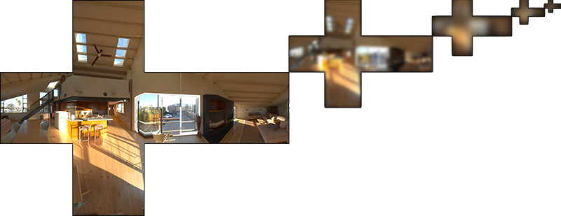
The result of the calculation of the first part is usually called the pre-filtered environment map , and is the environment map subjected to the convolution process specified by this expression. All this is similar to the process of obtaining an irradiance map, but in this case the convolution is carried out taking into account the roughness value. High roughness values ​​lead to the use of more disparate sampling vectors during the convolution process, which leads to more blurred results. The result of the convolution for each next selected level of roughness is stored in the next mip level of the prepared map of the environment. For example, an environment map that has been convolved for five different levels of roughness contains five mip levels and looks like this:


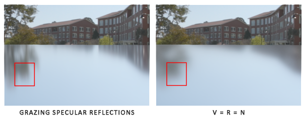
Sample vectors and their spread values ​​are determined based on the normal distribution function ( NDF ) of the BRDF Cook-Torrens model. This function takes the normal vector and the direction of observation as input parameters. Since the direction of observation is not known in advance at the time of preliminary calculation, the developers of Epic Games had to make one more assumption: the direction of gaze (and hence the direction of mirror reflection) is always identical to the output direction of the sample $$$\ omega_o$ . In the form of code:

vec3 N = normalize(w_o); vec3 R = N; vec3 V = R; 

In such conditions, the direction of gaze is not required in the process of convolving the environment map, which makes the calculation feasible in real time. But on the other hand, we lose the characteristic distortion of the mirror reflections when observed at an acute angle to the reflecting surface, as seen in the image below (from the publication Moving Frostbite to PBR ). In general, such a compromise is considered acceptable.


The second part of the split sum expression contains the BRDF of the original expression for the mirror component. Assuming that the incoming energy brightness is spectrally represented by white light for all directions (i.e., $$$L (p, x) = 1.0$ ), it is possible to pre-calculate the value for BRDF with the following input parameters: material roughness and honey angle normal $$$n$ and the direction of light $$$\ omega_i$ (or $$$n \ cdot \ omega_i$ ). The Epic Games approach involves storing the results of a BRDF calculation for each combination of roughness and angle between the normal and the direction of light in the form of a two-dimensional texture known as the BRDF ( BRDF integration map ), which is later used as a look-up table . This reference texture uses red and green output channels to store the scale and offset to calculate the surface Fresnel coefficient, which ultimately allows us to solve the second part of the expression for the split sum:


This auxiliary texture is created as follows: horizontal texture coordinates (ranging from [0., 1.]) are considered as values ​​of the input parameter $$$n \ cdot \ omega_i$ BRDF functions; Texture coordinates on a vertical are considered as input roughness values.

As a result, having such an integration map and a pre-processed environment map, you can combine samples from them to get the total value of the integral expression of the mirror component:

 float lod = getMipLevelFromRoughness(roughness); vec3 prefilteredColor = textureCubeLod(PrefilteredEnvMap, refVec, lod); vec2 envBRDF = texture2D(BRDFIntegrationMap, vec2(NdotV, roughness)).xy; vec3 indirectSpecular = prefilteredColor * (F * envBRDF.x + envBRDF.y) 

This review of the split-sum method from Epic Games should help create an impression of the process of approximate calculation of the part of the reflectivity that is responsible for the mirror component. Now we will try to prepare these maps on our own.

Pre-filtering HDR environment maps

The pre-filtering of the environment map proceeds in a similar way to what was done to obtain an irradiance map. The only difference is that now we take into account the roughness and save the result for each level of roughness in the new mip-level cubic map.

To begin with, you will have to create a new cubic map that will contain the result of the preliminary filtering. In order to create the required number of mip levels, we simply call glGenerateMipmaps () - the necessary memory will be allocated for the current texture:

 unsigned int prefilterMap; glGenTextures(1, &prefilterMap); glBindTexture(GL_TEXTURE_CUBE_MAP, prefilterMap); for (unsigned int i = 0; i < 6; ++i) { glTexImage2D(GL_TEXTURE_CUBE_MAP_POSITIVE_X + i, 0, GL_RGB16F, 128, 128, 0, GL_RGB, GL_FLOAT, nullptr); } glTexParameteri(GL_TEXTURE_CUBE_MAP, GL_TEXTURE_WRAP_S, GL_CLAMP_TO_EDGE); glTexParameteri(GL_TEXTURE_CUBE_MAP, GL_TEXTURE_WRAP_T, GL_CLAMP_TO_EDGE); glTexParameteri(GL_TEXTURE_CUBE_MAP, GL_TEXTURE_WRAP_R, GL_CLAMP_TO_EDGE); glTexParameteri(GL_TEXTURE_CUBE_MAP, GL_TEXTURE_MIN_FILTER, GL_LINEAR_MIPMAP_LINEAR); glTexParameteri(GL_TEXTURE_CUBE_MAP, GL_TEXTURE_MAG_FILTER, GL_LINEAR); glGenerateMipmap(GL_TEXTURE_CUBE_MAP); 

Note: since the prefilterMap selection will be conducted taking into account the existence of mip levels, it is necessary to set the reduction filter mode to GL_LINEAR_MIPMAP_LINEAR mode to enable trilinear filtering. Pre-processed images of mirror reflections are stored in separate faces of a cube map with a resolution at the base mip level of only 128x128 pixels. For most materials, this is quite enough, however, if you have an increased amount of smooth, shiny surfaces in your scene (for example, a new car), you may need to increase this resolution.

In the previous lesson, we convolved the environment map by creating sample vectors that are evenly distributed in the hemisphere. $$$\ Omega$ using spherical coordinates. For obtaining irradiance, this method is quite effective, which cannot be said about the calculations of specular reflections. The physics of specular highlights tells us that the direction of specularly reflected light is adjacent to the reflection vector. $$$r$ for surface with normal $$$n$ , even if the roughness is not zero:


The generalized form of the possible outgoing directions of reflection is called the mirror lobe ; the “ specular lobe of the mirror pattern” is perhaps too verbose, the reference point ). As the roughness increases, the petal grows and expands. Also, its shape changes depending on the direction of light falling. Thus, the shape of the petal strongly depends on the properties of the material.

Returning to the model of microsurfaces, you can imagine the shape of the mirror lobe as describing the orientation of the reflection relative to the median vector of the micro-surfaces, taking into account some given direction of light incidence. Realizing that most of the rays of the reflected light lies inside the mirror petal, oriented on the basis of the median vector, it makes sense to create a vector of the sample, oriented in a similar way. Otherwise, many of them will be useless. This approach is called importance sampling .

Monte Carlo integration and sampling by significance

To fully understand the essence of the sample in terms of significance, you will first have to become familiar with such a mathematical apparatus as the Monte-Carlo integration method. This method is based on a combination of statistics and probability theory and helps to carry out a numerical solution of a certain statistical problem on a large sample without the need to consider each element of this sample.

For example, you want to calculate the average growth of a country's population. To obtain an accurate and reliable result, one would have to measure the growth of every citizen and average the result. However, since the population of most countries is quite large, this approach is practically unrealizable, since it requires too many resources for implementation.
Another approach is to create a smaller subsample filled with truly random (unbiased) elements of the original sample. Next, you also measure growth and average the result for this subsample. You can take at least a hundred people and get a result, though not absolutely accurate, but still close enough to the real situation. The explanation for this method lies in the consideration of the law of large numbers. And its essence is described as follows: the result of a certain dimension in a smaller subsample size $$$N$ , composed of truly random elements of the original set, will be close to the control result of the measurement carried out on the entire original set. Moreover, the approximate result tends to true with increasing $$$N$ .
Monte-Carlo integration is an application of the law of large numbers to solve integrals. Instead of solving the integral taking into account the whole (possibly infinite) set of values $$$x$ , we use $$$N$ random sampling points and averaging the result. With growth $$$N$ the approximate result is guaranteed to approach the exact solution of the integral.

$$

$$O = \ int \ limits_ {a} ^ {b} f (x) dx = \ frac {1} {N} \ sum_ {i = 0} ^ {N-1} \ frac {f (x)} { pdf (x)}$$

To solve the integral, we obtain the value of the integrand for $$$N$ random points from a sample within [a, b], the results are summarized and divided by the total number of points taken for averaging. Element $$$pdf$ describes the probability density function , which shows how likely each selected value is found in the original sample. For example, this function for the growth of citizens would look like this:


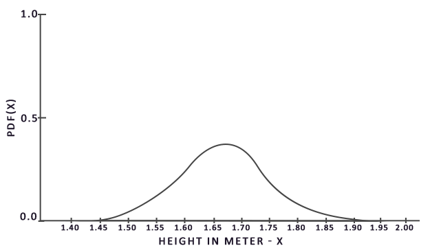
It can be seen that when using random sampling points, we have a much higher chance of meeting the height value of 170 cm than someone with a height of 150 cm.

It is clear that when carrying out Monte Carlo integration, some sample points are more likely to appear in sequence than others. Therefore, in any expression for the Monte Carlo estimate, we divide or multiply the selected value by the probability of its occurrence, using the probability density function. At the moment, when evaluating the integral, we created a set of uniformly distributed sampling points: the chance of obtaining any of them was the same. Thus, our estimate was unbiased , which means that as the number of sample points grows, our estimate will converge to the exact solution of the integral.

However, there are evaluation functions that are biased , i.e. implying the creation of sampling points not in a truly random manner, but with a predominance of a certain value or direction. Such evaluation functions allow Monte-Carlo evaluation to converge to an exact solution much faster . On the other hand, due to the bias of the evaluation function, the solution may never converge. In the general case, this is considered an acceptable compromise, especially in computer graphics tasks, since the estimate is very close to the analytical result and is not required if its effect looks quite reliably. As we will soon see sampling by significance (using an offset estimation function) allows you to create sample points shifted in a certain direction, which is taken into account by multiplying or dividing each selected value by the corresponding value of the probability density function.

Monte-Carlo integration is quite common in computer graphics tasks, since it is a fairly intuitive method for estimating the value of continuous integrals by a numerical method, which is quite effective. It is enough to take some area or volume in which the sample is taken (for example, our hemisphere $$$\ Omega$ ) create $$$N$ random sample points lying inside, and conduct a weighted summation of the obtained values.

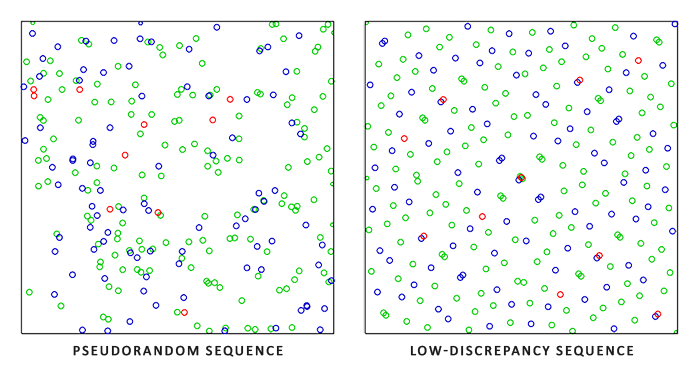
The Monte Carlo method is a very extensive topic for discussion, and here we will no longer go into details, but one more important detail remains: there is not a single way to create random samples . By default, each sample point is completely (random) random - which is what we expect. But, using certain properties of quasi-random sequences, it is possible to create sets of vectors that, although random, have interesting properties. For example, when creating random samples for the integration process, you can use the so-called low mismatch sequences ( low-discrepancy sequences ), which ensure the randomness of the created sample points, but in the total set they are more evenly distributed :


Using low-inconsistency sequences to create a set of sample vectors for the integration process is a quasi-Monte Carlo method ( Quasi-Monte Carlo intergration ). Monte Carlo quasi-methods converge much faster than the general approach, which is a very attractive feature for applications with high performance requirements.

So, we know about the general and quasi-Monte-Carlo method, but there is one more detail which will provide even greater convergence rate: sampling by significance.
As already noted in the lesson, for specular reflections, the direction of the reflected light is enclosed in a mirror lobe, the size and shape of which depends on the roughness of the reflecting surface. Understanding that any (quasi) random sampling vectors that are outside the mirror lobe will not affect the integral expression of the mirror component, i.e. are useless. It makes sense to focus the generation of sampling vectors in the region of the mirror lobe using the offset estimation function for the Monte Carlo method.

This is the essence of sampling by importance: the creation of sampling vectors lies in a certain area, oriented along the median vector of micro-surfaces, and the shape of which is determined by the roughness of the material. Using a combination of the quasi-Monte Carlo method, low-mismatch sequences and the displacement of the process of creating sample vectors due to sampling by significance, we achieve very high convergence rates. Since the convergence to the solution is fast enough, we can use a smaller number of sample vectors while still achieving a fairly reasonable estimate. The combination of methods described, in principle, allows graphic applications to even solve the integral of the mirror component in real time, although a preliminary calculation still remains a much more advantageous approach.

Low mismatch sequence

In this lesson, we still use the preliminary calculation of the mirror component of the expression of reflectivity for indirect radiation. And we will use the sampling by significance using a random sequence of low discrepancy and the quasi-Monte Carlo method. The sequence used is known as the Hammersley sequence ( Hammersley sequence ), a detailed description of which is given by Holger Dammertz . This sequence, in turn, is based on the van der Corput sequence ( van der Corput sequence ), which uses a special binary transform of the decimal relative to the decimal point.

Using cunning tricks of bitwise arithmetic, one can effectively define the van der Corput sequence directly in the shader and use it to create the i-th element of the Hammersley sequence from the sample to $$$N$ items:

 float RadicalInverse_VdC(uint bits) { bits = (bits << 16u) | (bits >> 16u); bits = ((bits & 0x55555555u) << 1u) | ((bits & 0xAAAAAAAAu) >> 1u); bits = ((bits & 0x33333333u) << 2u) | ((bits & 0xCCCCCCCCu) >> 2u); bits = ((bits & 0x0F0F0F0Fu) << 4u) | ((bits & 0xF0F0F0F0u) >> 4u); bits = ((bits & 0x00FF00FFu) << 8u) | ((bits & 0xFF00FF00u) >> 8u); return float(bits) * 2.3283064365386963e-10; // / 0x100000000 } // ---------------------------------------------------------------------------- vec2 Hammersley(uint i, uint N) { return vec2(float(i)/float(N), RadicalInverse_VdC(i)); } 

The Hammersley () function returns the i-th element of the low mismatch sequence from a set of size samples $$$N$ .

Not all OpenGL drivers support bitwise operations (WebGL and OpenGL ES 2.0, for example), so some environments might require an alternative implementation of their use:

 float VanDerCorpus(uint n, uint base) { float invBase = 1.0 / float(base); float denom = 1.0; float result = 0.0; for(uint i = 0u; i < 32u; ++i) { if(n > 0u) { denom = mod(float(n), 2.0); result += denom * invBase; invBase = invBase / 2.0; n = uint(float(n) / 2.0); } } return result; } // ---------------------------------------------------------------------------- vec2 HammersleyNoBitOps(uint i, uint N) { return vec2(float(i)/float(N), VanDerCorpus(i, 2u)); } 

I note that due to certain restrictions on the loop operators in the old hardware, this implementation runs through all 32 bits. As a result, this version is not as productive as the first option - but it works on any hardware and even in the absence of bit operations.

Sampling by importance in the GGX model

Instead of a uniform or random (Monte Carlo) distribution of the generated sample vectors within the hemisphere $$$\ Omega$ , appearing in the integral we are solving, we will try to create vectors so that they reflect the main direction of reflection of light, characterized by a median vector of microsurfaces and depending on the surface roughness. The sampling process itself will be similar to the previously considered one: open a cycle with a sufficiently large number of iterations, create an element of the low discrepancy sequence, use it to create a sampling vector in tangent space, transfer this vector to world coordinates and use it to sample the scene's energy brightness. In principle, the changes relate only to the fact that the element of the sequence of low discrepancies is now used to define the new sampling vector:

 const uint SAMPLE_COUNT = 4096u; for(uint i = 0u; i < SAMPLE_COUNT; ++i) { vec2 Xi = Hammersley(i, SAMPLE_COUNT); 

In addition, for the complete formation of the sample vector, it will be necessary in some way to orient it in the direction of the mirror petal corresponding to a given level of roughness. You can take the NDF (normal distribution function) from the lesson devoted to the theory and combine with the GGX NDF for the method of defining the vector of the sample in the field sponsored by Epic Games:

 vec3 ImportanceSampleGGX(vec2 Xi, vec3 N, float roughness) { float a = roughness*roughness; float phi = 2.0 * PI * Xi.x; float cosTheta = sqrt((1.0 - Xi.y) / (1.0 + (a*a - 1.0) * Xi.y)); float sinTheta = sqrt(1.0 - cosTheta*cosTheta); //       vec3 H; Hx = cos(phi) * sinTheta; Hy = sin(phi) * sinTheta; Hz = cosTheta; //        vec3 up = abs(Nz) < 0.999 ? vec3(0.0, 0.0, 1.0) : vec3(1.0, 0.0, 0.0); vec3 tangent = normalize(cross(up, N)); vec3 bitangent = cross(N, tangent); vec3 sampleVec = tangent * Hx + bitangent * Hy + N * Hz; return normalize(sampleVec); } 

The result is a sample vector, approximately oriented along the median vector of microsurfaces, for a given roughness and element of the sequence of low mismatch Xi . Note that Epic Games uses the square of the roughness value for greater visual quality, which is based on Disney’s original work on the PBR method.

After completing the implementation of the Hammersley sequence and the sample vector generation code, we can quote the prefilter and convolution shader code:

 #version 330 core out vec4 FragColor; in vec3 localPos; uniform samplerCube environmentMap; uniform float roughness; const float PI = 3.14159265359; float RadicalInverse_VdC(uint bits); vec2 Hammersley(uint i, uint N); vec3 ImportanceSampleGGX(vec2 Xi, vec3 N, float roughness); void main() { vec3 N = normalize(localPos); vec3 R = N; vec3 V = R; const uint SAMPLE_COUNT = 1024u; float totalWeight = 0.0; vec3 prefilteredColor = vec3(0.0); for(uint i = 0u; i < SAMPLE_COUNT; ++i) { vec2 Xi = Hammersley(i, SAMPLE_COUNT); vec3 H = ImportanceSampleGGX(Xi, N, roughness); vec3 L = normalize(2.0 * dot(V, H) * H - V); float NdotL = max(dot(N, L), 0.0); if(NdotL > 0.0) { prefilteredColor += texture(environmentMap, L).rgb * NdotL; totalWeight += NdotL; } } prefilteredColor = prefilteredColor / totalWeight; FragColor = vec4(prefilteredColor, 1.0); } 

We pre-filter the environment map based on some specified roughness, the level of which varies for each mip level of the resulting cubic map (from 0.0 to 1.0), and the result of the filter is stored in the variable prefilteredColor . Further, the variable is divided by the total weight for the entire sample, and samples with a smaller contribution to the final result (having a smaller NdotL value ) also increase the final weight less.

Preservation of pre-filtering data in mip levels

It remains to write the code directly instructing OpenGL to filter the environment map with different levels of roughness and then save the results in a series of mip levels of the target cubic map. Here, the code already prepared from the lesson on the calculation of the irradiance map will come in handy :

 prefilterShader.use(); prefilterShader.setInt("environmentMap", 0); prefilterShader.setMat4("projection", captureProjection); glActiveTexture(GL_TEXTURE0); glBindTexture(GL_TEXTURE_CUBE_MAP, envCubemap); glBindFramebuffer(GL_FRAMEBUFFER, captureFBO); unsigned int maxMipLevels = 5; for (unsigned int mip = 0; mip < maxMipLevels; ++mip) { //        - unsigned int mipWidth = 128 * std::pow(0.5, mip); unsigned int mipHeight = 128 * std::pow(0.5, mip); glBindRenderbuffer(GL_RENDERBUFFER, captureRBO); glRenderbufferStorage(GL_RENDERBUFFER, GL_DEPTH_COMPONENT24, mipWidth, mipHeight); glViewport(0, 0, mipWidth, mipHeight); float roughness = (float)mip / (float)(maxMipLevels - 1); prefilterShader.setFloat("roughness", roughness); for (unsigned int i = 0; i < 6; ++i) { prefilterShader.setMat4("view", captureViews[i]); glFramebufferTexture2D(GL_FRAMEBUFFER, GL_COLOR_ATTACHMENT0, GL_TEXTURE_CUBE_MAP_POSITIVE_X + i, prefilterMap, mip); glClear(GL_COLOR_BUFFER_BIT | GL_DEPTH_BUFFER_BIT); renderCube(); } } glBindFramebuffer(GL_FRAMEBUFFER, 0); 

The process is similar to the convolution of the irradiance map, but this time it is necessary at each step to clarify the size of the frame buffer, reducing it twice to match the mip levels. Also, the mip level to which the render will be conducted at the moment must be specified as a parameter of the function glFramebufferTexture2D () .

The result of the execution of this code should be a cubic map containing more and more blurred images of reflections on each subsequent mip level. You can use such a cubic map as a data source for a skybox and take a sample from any mip level to below zero:

 vec3 envColor = textureLod(environmentMap, WorldPos, 1.2).rgb; 

The result of this action will be the following picture:


Looks like a very blurred source environment map. If you have a similar result, then, most likely, the process of pre-filtering the HDR environment map is correct. Try experimenting with a selection of different mip levels and observe a gradual increase in blurring with each level.

Prefilter convolution artifacts

For most tasks, the described approach works quite well, but sooner or later you will have to meet with various artifacts that the pre-filtering process generates. Here are the most common and methods of dealing with them.

The manifestation of the seams of the cubic card

Sampling values ​​from a pre-filtered cubic map for surfaces with high roughness leads to reading data from the mip level somewhere near the end of their chain. When sampling from a cube map, OpenGL does not, by default, perform linear interpolation between the faces of a cube map. Since high mip-levels have a lower resolution, and the environment map has been convolved, taking into account the very large mirror lobe, the lack of texture filtering between the faces becomes obvious:


Fortunately, OpenGL has the ability to activate such filtering with a simple flag:

 glEnable(GL_TEXTURE_CUBE_MAP_SEAMLESS); 

It is enough to set the flag somewhere in the application initialization code and this artifact is over.

The appearance of bright spots

Since the specular reflections in general contain high-frequency details, as well as areas with very different brightness, their convolution requires the use of a large number of sample points to correctly take into account the large scatter of values ​​within the HDR reflections from the environment. In the example, we already take a sufficiently large number of samples, but for certain scenes and high levels of roughness of the material, this still will not be enough, and you will witness the appearance of many spots around bright areas:


You can continue to increase the number of samples, but it will not be a universal solution and in some conditions it will still allow an artifact. But you can refer to the method Chetan Jags , which allows to reduce the manifestation of the artifact. To do this, at the preliminary convolution stage, the sample from the environment map should not be directly taken, but from one of its mip levels, based on the value obtained from the probability distribution function of the integrand expression and roughness:

 float D = DistributionGGX(NdotH, roughness); float pdf = (D * NdotH / (4.0 * HdotV)) + 0.0001; //        float resolution = 512.0; float saTexel = 4.0 * PI / (6.0 * resolution * resolution); float saSample = 1.0 / (float(SAMPLE_COUNT) * pdf + 0.0001); float mipLevel = roughness == 0.0 ? 0.0 : 0.5 * log2(saSample / saTexel); 

Just do not forget to enable trilinear filtering for the environment map in order to successfully sample from mip levels:

 glBindTexture(GL_TEXTURE_CUBE_MAP, envCubemap); glTexParameteri(GL_TEXTURE_CUBE_MAP, GL_TEXTURE_MIN_FILTER, GL_LINEAR_MIPMAP_LINEAR); 

Also, do not forget to create the texture mip levels directly using OpenGL, but only after the main mip level is fully formed:

 //  HDR      ... [...] //  - glBindTexture(GL_TEXTURE_CUBE_MAP, envCubemap); glGenerateMipmap(GL_TEXTURE_CUBE_MAP); 

This method works surprisingly well, removing almost all (and often all) spots on the filtered map, even at high levels of roughness.

Preliminary calculation of BRDF

So, we have successfully processed the environment map with a filter and now we can concentrate on the second part of the approximation in the form of a separate amount, which is BRDF. To refresh your memory, look again at the complete record of the approximate solution:

$$

$$L_o(p,\omega_o) = \int\limits_{\Omega} L_i(p,\omega_i) d\omega_i * \int\limits_{\Omega} f_r(p, \omega_i, \omega_o) n \cdot \omega_i d\omega_i$$

We preliminarily calculated the left part of the sum and wrote the results for different levels of roughness into a separate cubic map. The right side will require convolving the BDRF expression together with the following parameters: angle$$n ⋅ ω i , surface roughness and Fresnel coefficient$n \cdot \omega_i$$$$F_0$ . A process similar to the integration of a mirrored BRDF for a completely white environment or with constant energy brightness $$$L_i = 1.0$ . BRDF convolution for three variables is not a trivial task, but in this case $$F 0 can be derived from an expression describing a BRDF mirror:$F_0$

$$

$$\int\limits_{\Omega} f_r(p, \omega_i, \omega_o) n \cdot \omega_i d\omega_i = \int\limits_{\Omega} f_r(p, \omega_i, \omega_o) \frac{F(\omega_o, h)}{F(\omega_o, h)} n \cdot \omega_i d\omega_i$$

Here $$F - a function describing the calculation of the Fresnel kit. By moving the divisor to the expression for BRDF, you can go to the following equivalent entry:$F$

$$

$$\int\limits_{\Omega} \frac{f_r(p, \omega_i, \omega_o)}{F(\omega_o, h)} F(\omega_o, h) n \cdot \omega_i d\omega_i$$

Replacing the right entry $$F to the Fresnel-Schlick approximation, we get:$F$

$$

$$\int\limits_{\Omega} \frac{f_r(p, \omega_i, \omega_o)}{F(\omega_o, h)} (F_0 + (1 - F_0){(1 - \omega_o \cdot h)}^5) n \cdot \omega_i d\omega_i$$

Denote the expression $$${(1 - \omega_o \cdot h)}^5$ as $$/ a l p h a to simplify the decision regarding$/alpha$$$$F_0$ :

$$

$$\int\limits_{\Omega} \frac{f_r(p, \omega_i, \omega_o)}{F(\omega_o, h)} (F_0 + (1 - F_0)\alpha) n \cdot \omega_i d\omega_i$$

$$

$$\int\limits_{\Omega} \frac{f_r(p, \omega_i, \omega_o)}{F(\omega_o, h)} (F_0 + 1*\alpha - F_0*\alpha) n \cdot \omega_i d\omega_i$$

$$

$$\int\limits_{\Omega} \frac{f_r(p, \omega_i, \omega_o)}{F(\omega_o, h)} (F_0 * (1 - \alpha) + \alpha) n \cdot \omega_i d\omega_i$$

Further function $$F we divide into two integrals:$F$

$$

$$\int\limits_{\Omega} \frac{f_r(p, \omega_i, \omega_o)}{F(\omega_o, h)} (F_0 * (1 - \alpha)) n \cdot \omega_i d\omega_i + \int\limits_{\Omega} \frac{f_r(p, \omega_i, \omega_o)}{F(\omega_o, h)} (\alpha) n \cdot \omega_i d\omega_i$$

In this way $$F 0 will be constant under the integral, and we can take it beyond the integral sign. Next, we will reveal$F_0$$$α in the original expression and get the final entry for BRDF as a split amount:$\alpha$

$$

$$F_0 \int\limits_{\Omega} f_r(p, \omega_i, \omega_o)(1 - {(1 - \omega_o \cdot h)}^5) n \cdot \omega_i d\omega_i + \int\limits_{\Omega} f_r(p, \omega_i, \omega_o) {(1 - \omega_o \cdot h)}^5 n \cdot \omega_i d\omega_i$$

The resulting two integrals represent the scale and offset for the value $$$F_0$ respectively. Notice that $$f ( p , ω i , ω o ) contains the occurrence$f(p, \omega_i, \omega_o)$$$F , therefore these occurrences cancel each other out and disappear from the expression. Using the already developed approach, we can carry out the BRDF convolution together with the input data: roughness and angle between vectors$F$

$$$n$ and $$$w_o$ .Write the result in the 2D texture - card complexation BRDF ( BRDF integration map ), which will serve as an auxiliary table values for use in the final shader, which will form the final result of the indirect specular lighting.

The BRDF convolution shader works on a plane, directly using two-dimensional texture coordinates as inputs to the convolution process ( NdotV and roughness ). The code is noticeably similar to the convolution convolution, but here the sample vector is processed taking into account the BRDF geometric function and the Fresnel-Schlick approximation expression:

 vec2 IntegrateBRDF(float NdotV, float roughness) { vec3 V; Vx = sqrt(1.0 - NdotV*NdotV); Vy = 0.0; Vz = NdotV; float A = 0.0; float B = 0.0; vec3 N = vec3(0.0, 0.0, 1.0); const uint SAMPLE_COUNT = 1024u; for(uint i = 0u; i < SAMPLE_COUNT; ++i) { vec2 Xi = Hammersley(i, SAMPLE_COUNT); vec3 H = ImportanceSampleGGX(Xi, N, roughness); vec3 L = normalize(2.0 * dot(V, H) * H - V); float NdotL = max(Lz, 0.0); float NdotH = max(Hz, 0.0); float VdotH = max(dot(V, H), 0.0); if(NdotL > 0.0) { float G = GeometrySmith(N, V, L, roughness); float G_Vis = (G * VdotH) / (NdotH * NdotV); float Fc = pow(1.0 - VdotH, 5.0); A += (1.0 - Fc) * G_Vis; B += Fc * G_Vis; } } A /= float(SAMPLE_COUNT); B /= float(SAMPLE_COUNT); return vec2(A, B); } // ---------------------------------------------------------------------------- void main() { vec2 integratedBRDF = IntegrateBRDF(TexCoords.x, TexCoords.y); FragColor = integratedBRDF; } 

As can be seen, the BRDF convolution is implemented in the form of a practically literal arrangement of the above mathematical calculations. Take the input parameters of roughness and angle$$θ , the sample vector is generated based on a sample of significance, processed using the geometry function and the converted Fresnel expression for BRDF. As a result, for each sample, we obtain the magnitude of the scaling and offset values$\theta$$$F 0 , which at the end are averaged and returned asvec2. In thetheoreticallesson it was mentioned that the geometric component of BRDF is slightly different in the case of calculating IBL, since the coefficient$F_0$

$$k is set differently:$k$

$$

$$k_{direct} = \frac{(\alpha + 1)^2}{8}$$

$$

$$k_{IBL} = \frac{\alpha^2}{2}$$

Since the BRDF convolution is part of the solution of the integral in the case of calculating IBL, we will use the coefficient $$k I B L to calculate the geometry function in the Schlick-GGX model:$k_{IBL}$

 float GeometrySchlickGGX(float NdotV, float roughness) { float a = roughness; float k = (a * a) / 2.0; float nom = NdotV; float denom = NdotV * (1.0 - k) + k; return nom / denom; } // ---------------------------------------------------------------------------- float GeometrySmith(vec3 N, vec3 V, vec3 L, float roughness) { float NdotV = max(dot(N, V), 0.0); float NdotL = max(dot(N, L), 0.0); float ggx2 = GeometrySchlickGGX(NdotV, roughness); float ggx1 = GeometrySchlickGGX(NdotL, roughness); return ggx1 * ggx2; } 

Note that the coefficient $$k is calculated based on the parametera. In this case, theroughnessparameter isnot squared when describing the parametera, which was done in other places where this parameter was applied. Not sure where the problem lies here: the Epic Games or in the original work by Disney, but it is worth saying that it is a direct assignment of the value ofroughnessparameteraleads to the creation of maps integration BRDF identical, presented in the publication of Epic Games.Further, the preservation of the BRDF convolution results will be provided in the form of a 2D texture of size 512x512:$k$

 unsigned int brdfLUTTexture; glGenTextures(1, &brdfLUTTexture); //   ,     glBindTexture(GL_TEXTURE_2D, brdfLUTTexture); glTexImage2D(GL_TEXTURE_2D, 0, GL_RG16F, 512, 512, 0, GL_RG, GL_FLOAT, 0); glTexParameteri(GL_TEXTURE_2D, GL_TEXTURE_WRAP_S, GL_CLAMP_TO_EDGE); glTexParameteri(GL_TEXTURE_2D, GL_TEXTURE_WRAP_T, GL_CLAMP_TO_EDGE); glTexParameteri(GL_TEXTURE_2D, GL_TEXTURE_MIN_FILTER, GL_LINEAR); glTexParameteri(GL_TEXTURE_2D, GL_TEXTURE_MAG_FILTER, GL_LINEAR); 

As recommended by Epic Games, the 16-bit floating point format is used here. Be sure to set the repeat mode to GL_CLAMP_TO_EDGE to avoid sampling artifacts from the edge.

Next, we use the same frame buffer object and execute the shader on the full-screen quad surface:

 glBindFramebuffer(GL_FRAMEBUFFER, captureFBO); glBindRenderbuffer(GL_RENDERBUFFER, captureRBO); glRenderbufferStorage(GL_RENDERBUFFER, GL_DEPTH_COMPONENT24, 512, 512); glFramebufferTexture2D(GL_FRAMEBUFFER, GL_COLOR_ATTACHMENT0, GL_TEXTURE_2D, brdfLUTTexture, 0); glViewport(0, 0, 512, 512); brdfShader.use(); glClear(GL_COLOR_BUFFER_BIT | GL_DEPTH_BUFFER_BIT); RenderQuad(); glBindFramebuffer(GL_FRAMEBUFFER, 0); 

As a result, we obtain a texture map that stores the result of the convolution of the part of the expression for the separate amount responsible for BRDF:


Having on hand the results of the preliminary filtering of the environment map and the texture with the results of the BRDF convolution, we will be able to restore the result of calculating the integral for indirect specular illumination based on approximation by a separate sum. The recovered value will subsequently be used as indirect or background specular radiation.

The final calculation of reflectivity in the IBL model

So, to get the value that describes the indirect mirror component in the general expression of reflectivity, it is necessary to “glue” the calculated approximation components into a single whole by a separate sum. First, add the appropriate samplers for the pre-calculated data to the final shader:

 uniform samplerCube prefilterMap; uniform sampler2D brdfLUT; 

First, we obtain the value of indirect mirror reflection on the surface by sampling from a previously processed environment map based on the reflection vector. Note that here the selection of the mip level for sampling is based on the surface roughness. For rougher surfaces, the reflection will be more blurred :

 void main() { [...] vec3 R = reflect(-V, N); const float MAX_REFLECTION_LOD = 4.0; vec3 prefilteredColor = textureLod(prefilterMap, R, roughness * MAX_REFLECTION_LOD).rgb; [...] } 

At the preliminary convolution stage, we prepared only 5 mip levels (from zero to fourth); the MAX_REFLECTION_LOD constant serves to limit the sample of the generated mip levels.

Next, we make a sample of the BRDF integration map based on the roughness and angle between the normal and the direction of gaze:

 vec3 F = FresnelSchlickRoughness(max(dot(N, V), 0.0), F0, roughness); vec2 envBRDF = texture(brdfLUT, vec2(max(dot(N, V), 0.0), roughness)).rg; vec3 specular = prefilteredColor * (F * envBRDF.x + envBRDF.y); 

The value obtained from the map contains the scaling and offset factors for the value $$F 0 (here the valueFistaken- Fresnel coefficient). The converted valueF isthen combined with the value obtained from the pre-filtering map to obtain an approximate solution to the original integral expression —specular.In this way, we get a solution for the part of the reflectivity that is responsible for the specular reflection. To obtain a complete solution of the PBR IBL model, it is necessary to combine this value with the solution for the diffuse part of the reflectivity we received in thelastlesson:$F_0$

 vec3 F = FresnelSchlickRoughness(max(dot(N, V), 0.0), F0, roughness); vec3 kS = F; vec3 kD = 1.0 - kS; kD *= 1.0 - metallic; vec3 irradiance = texture(irradianceMap, N).rgb; vec3 diffuse = irradiance * albedo; const float MAX_REFLECTION_LOD = 4.0; vec3 prefilteredColor = textureLod(prefilterMap, R, roughness * MAX_REFLECTION_LOD).rgb; vec2 envBRDF = texture(brdfLUT, vec2(max(dot(N, V), 0.0), roughness)).rg; vec3 specular = prefilteredColor * (F * envBRDF.x + envBRDF.y); vec3 ambient = (kD * diffuse + specular) * ao; 

I note that the specular value does not multiply by kS , since it already contains the Fresnel coefficient.

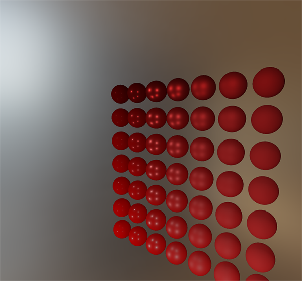
Let us launch our test application with a familiar set of spheres with varying metallicity and roughness characteristics and take a look at their appearance in full magnificence of PBR:


You can go even further and download a set of textures corresponding to the PBR model and get the spheres from real materials :


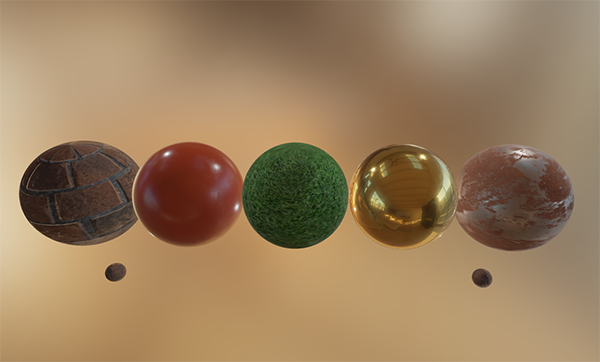
Or even download a smart model along with Andrew Maximov’s prepared PBR textures :


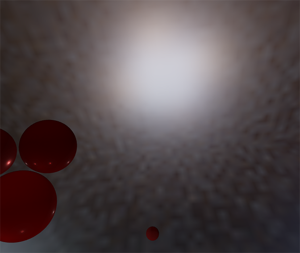
I think that no one should be particularly convinced that the current lighting model looks much more convincing. Moreover, the lighting looks physically correct, regardless of the environment map. Below are used several completely different HDR environment maps that completely change the nature of the lighting - but all the images look physically reliable, despite the fact that no parameters were needed in the model! (In principle, this simplification of work with materials is the main plus of the PBR pipeline, and a better picture can be said to be a pleasant consequence. Approx. Per. )


Phew, our journey into the essence of the PBR render came out pretty voluminous. We went through the whole series of short steps to the result and, of course, a lot can go wrong with the first approaches. Therefore, in case of any problems, I advise you to carefully understand the code of examples for monochrome and texturized spheres (and the shader code, of course!). Or ask for advice in the comments.

What's next?

I hope that by reading these lines you have already made out for yourself an understanding of the work of the PBR model of the render, and also figured out and successfully launched a test application. In these lessons, all the necessary auxiliary texture maps for the PBR model were calculated in our application in advance, before the main render cycle. For learning tasks, this approach is suitable, but not for practical use. First, such preliminary preparation should occur once, and not every application launch. Secondly, if you decide to add some more environment maps, they will also have to be processed at startup. And if some more cards are added? This snowball.

That is why, in general, the irradiance map and the pre-processed environment map are prepared once and then saved on disk (the BRDF integration map does not depend on the environment map, so that it can be calculated or loaded once). It follows that you will need a format for storing HDR cubic cards, including their mip levels. Well, or you can store and load them using one of the widespread formats (this way .dds supports saving mip levels).

Another important point: in order to give a deep understanding of the PBR pipeline in these lessons, I gave a description of the full process of preparing for the PBR renderer, including preliminary calculations of auxiliary cards for IBL. However, in your practice, you might as well use one of the great utilities that will prepare these cards for you: for example, cmftStudio or IBLBaker .

We also did not consider the process of preparing cubic reflection reflection samples ( reflection probes) and the associated processes of interpolation of cubic maps and parallax correction. Briefly, this technique can be described as follows: we place in our scene a set of objects of reflection samples, which form a local environment picture in the form of a cubic map, and then on the basis of it all the necessary auxiliary maps for the IBL model are formed. By interpolating data from several samples based on the distance from the camera, you can get highly detailed lighting based on the image, the quality of which is essentially limited only by the number of samples that we are ready to place in the scene. This approach allows the lighting to change correctly, for example, when moving from a brightly lit street to the dusk of a certain room. I’ll probably write a lesson about reflection samples in the future,however, at the moment I can only recommend for review the article by Chetan Jags, given below.

(Implementation of samples, and much more can be found in the raw materials of the author of the author of tutorials here , comment. Per. )

Additional materials

1. Real Shading in Unreal Engine 4 : Clarification of the Epic Games approach to approximating the expression for the mirror component by a separate sum. Based on this article, the code for the IBL PBR lesson was designed.
2. Physically Based Shading and Image Based Lighting : An excellent article describing the process of incorporating the calculation of the mirror component of IBL into a PBR Pipeline interactive application.
3. Image Based Lighting : a very voluminous and detailed post about mirror IBL and related issues, including the task of light probe interpolation.
4. Moving Frostbite to PBR : , PBR «AAA».
5. Physically Based Rendering – Part Three : , IBL PBR JMonkeyEngine.
6. Implementation Notes: Runtime Environment Map Filtering for Image Based Lighting : HDR , .