Let's remove quaternions from all 3D engines.
For recording three-dimensional turns, graphics programmers use quaternions . However, quaternions are difficult to understand, because they are studied superficially . We just take on faith strange multiplication tables and other mysterious definitions, and use them as “black boxes”, turning vectors as we need. Why m a t h b f i 2 = m a t h b f j 2 = m a t h b f k 2 = - 1 and m a t h b f i m a t h b f j = m a t h b f k ? Why do we take a vector and turn it into an “imaginary” vector to transform it, for example mathbfq(x mathbfi+y mathbfj+z mathbfk) mathbfq∗ ? But who cares if everything works, right?
There is a way of describing turns called a rotor , which belongs to a region and complex numbers (in 2D), and quaternions (in 3D), and even generalizes to any number of dimensions.
We can create rotors almost completely from scratch , instead of determining quaternions from nothing and trying to explain how they work in hindsight . It takes more time, but it seems to me that it is worth it, because they are much easier to understand!
')
In addition, to visualize and understand the three-dimensional rotors do not need to use the fourth spatial dimension.
It would be great if they began to force out the use and study of quaternions, replacing them with rotors. It is very easy to replace them, and the code will remain almost the same . Everything that can be done with quaternions, for example, interpolation and elimination of axis locking (Gimbal lock), can be done with rotors. But we begin to understand much more.
(In the original article, all the graphics are interactive, and the article is followed by a video. By clicking on the play buttons, you can launch the corresponding section of the video. You can also click the transition button below the video to go to the corresponding section of the article. You can maximize the window so that the video has more space , or set a constant size for it.)
1. Planes of turns
1.1. Turns are performed on two-dimensional planes.
In three-dimensional space, we usually perceive turns as occurring around axles, as the wheel rotates on an axis, but instead it would be more correct to represent the plane on which the wheel lies. This plane is perpendicular to the axis.
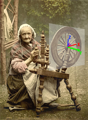
This old woman spins the wheel in the plane mathbfxz perpendicular to the axis mathbfy .
This happens because if we divide the vector into two parts, one of which lies on the plane ( mathbfv parallel ), and the other is outside ( mathbfv perp ), then the rotation rotates the inner part, and the outer remains unchanged.

Rotate in the plane yx [ in the original article this is animation and the camera can be moved ]
In two-dimensional space there is only one plane in which rotation is possible ( there is no outer part ). Therefore, to assume that turns occur around the third axis (perpendicular to the 2D plane) is strictly speaking wrong, because for performing turns we do not need to add another dimension.
If you tell a two-dimensional “planter” (who lives inside a 2D-plane and never gets out of two-dimensional space) about a perpendicular axis of rotation, he would ask: “In what direction does this axis point? I can't imagine her! ”
And in higher dimensions (4D and above) it is impossible to determine one vector of the normal to the 2D plane (for example, in 4D the 2D plane has two directions of normals, in 5D there are three directions of normals, and n D their n - 2 )
1.2. The exact direction of turns
In addition, when we think about turning around an axis, the direction of turning is not defined, and therefore it should be determined by a rule (the so-called “right-hand rule”).
However, if we assume that the turns occur inside the planes, then the direction becomes clear: a turn in the plane mathbfxy means a turn that moves a (unit) vector mathbfx to (single) vector mathbfy inside the plane that they together form. Rotate in the plane mathbfyx - this is a reverse rotation: it moves the vector mathbfy to vector mathbfx .
I remember that when I first learned about the three matrices of 3D turns along orthogonal planes, I first thought: what the hell is the matrix m a t h b f R y has the opposite sign? So it turns out because of the rule of the right hand, according to which we must determine the rotation around the axis m a t h b f y so that it runs from mathbfz to mathbfx and not from mathbfx to mathbfz , to maintain a constant "right-handed" direction of rotation. When we start talking directly about the plane itself, this rule becomes unnecessary.R_X (\ theta) = \ begin {bmatrix} 1 & 0 & 0 \\ 0 & cos (\ theta) & -sin (\ theta) \\ 0 & sin (\ theta) & cos (\ theta) \ end {bmatrix} \: \: \: R_Y (\ theta) = \ begin {bmatrix} cos (\ theta) & 0 & \ bbox [5px, border-bottom: 2px solid red] {\ \} sin (\ theta) \\ 0 & 1 & 0 \\ \ bbox [5px, border-bottom: 2px solid red] {-} sin (\ theta) & 0 & cos (\ theta) \ end {bmatrix} \: \: \: R_Z (\ theta) = \ begin {bmatrix} cos (\ theta) & -sin (\ theta) & 0 \\ sin (\ theta) & cos (\ theta) & 0 \\ 0 & 0 & 1 \ end {bmatrix }
2. Bivektory
2.1. External product
To calculate the rotation axis when turning one vector mathbfa to another vector mathbfb we take the vector product of two vectors to get a vector perpendicular to both of them. But why should we “leave” the plane if the turn is essentially a two-dimensional operation?
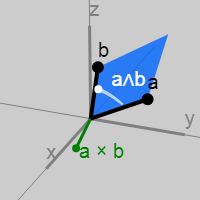
Instead, we take what is called an outer product (also known as a two-dimensional vector product) of two vectors, creating a new element called a “bivector” (or 2-vector) mathbfB representing the plane that the two vectors together form. If the vector product creates a vector normal to the plane, then the external product creates the plane itself . Calculating the plane normal is irrelevant.
mathbfB= mathbfa wedge mathbfb
mathbfB can be represented as a parallelogram constructed from vectors mathbfa and mathbfb in the plane that they together form.
At first, the idea of a bivector may seem strange, but soon we will see that they are almost as fundamental as the vectors themselves . If a vector can be compared with a straight line, then the bivector is similar to a plane ... The properties of the external product capture the important properties of the planes.
2.2. Basis for bivectors

Bivectors, like vectors, have components. But they are defined on the basis of planes , not straight lines , like vectors.
Three orthogonal basal planes are mathbfx wedge mathbfy , mathbfx wedge mathbfz and mathbfy wedge mathbfz as we see from the figure.
But first, let's consider a simpler two-dimensional case ...
2.3. 2D bivectors
In 2D, there is only one plane, namely mathbfxy . That is, a two-dimensional bivector has only one component. For a bivector composed of vectors mathbfa and mathbfb this number Bxy equals the area (with sign) of the parallelogram formed by two vectors.
mathbfB= mathbfa wedge mathbfb=Bxy( mathbfx wedge mathbfy)
In the original article with a 2D bivector, you can experiment on interactive graphics by changing the (unit) vectors from which it is composed:
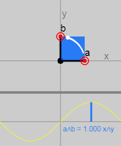
It can be seen that as the angle between the vectors changes, the area of the parallelogram changes (according to the sine of the angle).
If the vectors coincide or are parallel, then they do not form a regular plane and the result will be zero. This simple property defines what the bivector is:
mathbfa wedge mathbfa=0
Looking at the sum of two vectors, you can see that the property follows:
\ begin {eqnarray} (\ mathbf {a} + \ mathbf {b}) \ wedge (\ mathbf {a} + \ mathbf {b}) & = & 0 \\ \ mathbf {a} \ wedge \ mathbf { a} + \ mathbf {b} \ wedge \ mathbf {a} + \ mathbf {a} \ wedge \ mathbf {b} + \ mathbf {b} \ wedge \ mathbf {b} & = & 0 \\ \ mathbf { b} \ wedge \ mathbf {a} + \ mathbf {a} \ wedge \ mathbf {b} & = & 0 \ end {eqnarray}
Consequently:
mathbfa wedge mathbfb=− mathbfb wedge mathbfa
As well as the direction of rotation , the order of the arguments in the external work is important. Reversing the arguments changes the sign of the result (this is called "antisymmetry").
On the chart, the sign is indicated by a color that changes from blue to green. Sign changes when turning out mathbfa at mathbfb moves from a clockwise motion to a counterclockwise motion (i.e. if it corresponds to a direction (from mathbfx to mathbfy ) or direction (from mathbfy to mathbfx )).
It can be seen that the properties of the outer work are arranged in such a way that they transmit the properties of the planes and turns.
2.4. 2D bivectors from non-unit vectors
Obviously, the vectors do not need to be of unit length, and on this graph, this restriction is removed:

The area of the parallelogram with the sign is proportional to the lengths of both vectors: Bxy=sin( alpha) |a | |b | where alpha Is the angle between mathbfa and mathbfb . That is, for example, doubling the length of one vector doubles the area.
We can get the true value by substituting the vectors as components:
\ begin {eqnarray} \ mathbf {a} \ wedge \ mathbf {b} & = & (a_x \ mathbf {x} + a_y \ mathbf {y}) \ wedge (b_x \ mathbf {x} + b_y \ mathbf { y}) \\ & = & a_x b_x (\ mathbf {x} \ wedge \ mathbf {x}) + a_x b_y (\ mathbf {x} \ wedge \ mathbf {y}) + a_y b_x (\ mathbf {y} \ wedge \ mathbf {x}) + a_y b_y (\ mathbf {y} \ wedge \ mathbf {y}) \\ & = & a_x b_y (\ mathbf {x} \ wedge \ mathbf {y}) + a_y b_x ( \ mathbf {y} \ wedge \ mathbf {x}) \\ & = & a_x b_y (\ mathbf {x} \ wedge \ mathbf {y}) - a_y b_x (\ mathbf {x} \ wedge \ mathbf {y} ) \\ & = & (a_x b_y - a_y b_x) (\ mathbf {x} \ wedge \ mathbf {y}) \ end {eqnarray}
Bxy=axby−bxay
2.5. 3D bivectors

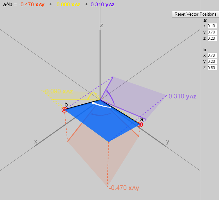
Same as vector coordinates mathbfv can be considered as projections of the vector onto three orthogonal basis axes ( mathbfx , mathbfy , mathbfz ) bivector coordinates mathbfB can be considered as projections smaller than a plane onto three orthogonal basal planes.
The projections of the vector are the lengths of this vector along each basis vector, and the projections of the bivector are the areas of the plane on each basis plane.
For a vector:
mathbfv= bbox[5px,border−bottom:2pxsolidred]vx mathbfx+ bbox[5px,border−bottom:2pxsolidgreen]vy mathbfy+ bbox[5px,border−bottom:2pxsolidblue]vz mathbfz
For the bivector:
mathbfB= bbox[5px,border−bottom:2pxsolidcoral]Bxy( mathbfx wedge mathbfy)+ bbox[5px,border−bottom:2pxsolidgold]Bxz( mathbfx wedge mathbfz)+ bbox[5px,border−bottom:2pxsolidDarkViolet]Byz( mathbfy wedge mathbfz)
Where Bxy , Bxz , Byz - it's just numbers, like vx , vy , vz (they are underlined by colors corresponding to the colors on the graphic).
The components of a 3D bivector are simply three 2D projections of the bivector on the basic 2D planes.
Using the same method as before, we find that the true values of the components look much like the XY component from the two-dimensional case, but applied to all three planes:
Bxy=axby−bxay
Bxz=axbz−bxaz
Byz=aybz−byaz
You can experiment with the 3D bivector on the interactive graphics in the original article:
Norm bivektora | mathbfB |= | mathbfa wedge mathbfb | is determined in the same way as the vector norm (the square root of the sum of the squares of the components). This is equal to the area of the parallelogram formed mathbfa and mathbfb i.e. | mathbfa wedge mathbfb |= midsin( alpha) mid | mathbfa | | mathbfb | where alpha - the angle between mathbfa and mathbfb .
If we divide the bivector by its norm, then we reduce two lengths of the vectors and the (absolute) value of the sine of the angle, that is, we will have a bivector. hat mathbfB which will be constructed as if the two vectors were originally perpendicular and had a unit length. This is a very clean representation of the plane containing both vectors. So:
mathbfB=| mathbfa | | mathbfb | midsin( alpha) mid hat mathbfB
Do you recall anything external work? In 3D, the definition of an external work is very similar to the definition of a vector product. In fact, a vector in 3D, obtained from a vector product (for example, a normal vector) will have three components equal to the components of a bivector (the numbers will be the same, but the basis is different).
$$ display $$ \ begin {eqnarray} \ mathbf {a} \ wedge \ mathbf {b} & = & & (a_x b_y - b_x a_y) (\ mathbf {x} \ wedge \ mathbf {y}) \\ & & + & (a_x b_z - b_x a_z) (\ mathbf {x} \ wedge \ mathbf {z}) \\ & & + & (a_y b_z - b_y a_z) (\ mathbf {y} \ wedge \ mathbf {z} ) \\ \\ \ mathbf {a} \ times \ mathbf {b} & = & & (a_x b_y - b_x a_y) \ \ mathbf {z} \\ & & - & (a_x b_z - b_x a_z) \ \ mathbf {y} \\ & & + & (a_y b_z - b_y a_z) \ \ mathbf {x} \ end {eqnarray} $$ display $$
The definition of a bivector has a geometrical meaning, but does not appear from nowhere. I remember that when I studied vector art, I thought: “Why the hell does it return a vector whose length is equal to the area of the parallelogram formed by these two vectors? It seems so random. And why can we turn the area of a parallelogram into a vector length ? ”
2.6. The semantics of vectors and bivectors
In 3D, a bivector has three coordinates, one per plane: ( mathbfxy , mathbfxz and mathbfyz ). Vectors also have three coordinates, one per axis ( mathbfx , mathbfy and mathbfz ). Each plane is perpendicular to one axis. This coincidence occurs only in three dimensions (*) and that is why we constantly confuse bivectors with vectors .
In 2D, there is only one basic bivector ( mathbfxy ), and in 3D there are 3 basic bivectors ( mathbfxy , mathbfxz , mathbfyz ), in 4D there are 6 basic bivectors ( mathbfxy , mathbfxz , mathbfxw , mathbfyz , mathbfyw , mathbfzw ) and so on...
In programming, they both have the same layout in memory, but different operations. Using a 3D vector instead of a 3D bivector is similar to the “type conversion” of a bivector.
Here is an example: you could see that normal vectors are transformed differently than ordinary vectors using the "inverse transfer" matrix ( mathbfMT)−1 , instead of the matrix itself. This happens because, in fact, they are actually not vectors, but bivectors, which have been transformed into vectors by “type conversion”. In physics, there is a hack called "axial vector", which was introduced in order to distinguish the vectors obtained by the vector product from the ordinary vectors. A bivector is a true “type” of an object and should be perceived and processed accordingly.
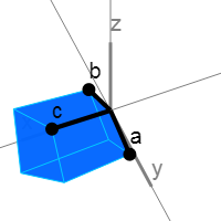
We can continue to take an external product to obtain not only oriented 2D-areas, but also oriented 3D-volumes. Trivector T can be obtained by performing an external work twice:mathbfT= mathbfa wedge mathbfb wedge mathbfc
In three-dimensional space, everything ends there. As in 2D, where there is only one plane that fills all the 2D space, in 3D there is only one volume that fills all the 3D space.
[But in nD we can continue to create even larger external products of vectors until we reach the nth dimension. For example, in 4D we have four basic trivectors (3-vectors) ( mathbfxyz , mathbfxyw , mathbfxwz , mathbfyzw ) and one basic 4-vector mathbfxyzw ]
In 3D, a trivector has only one basic component ( Txyz ), equal to the volume of the parallelepiped formed by three vectors. The triple outer product is an improved version of the scalar triple product ( ( mathbfa times mathbfb) cdot mathbfc ), because only one type of operation is involved in it, it returns the correct type (volume instead of scalar) and works in any number of measurements.mathbfT=Txyz mathbfx wedge mathbfy wedge mathbfz
3. Geometric product
3.1. Multiplication of vectors by each other
Geometric product mathbfab (denoted without a symbol) is another operation that can be performed with vectors. The geometric product is defined so that the vectors have inverse values (for example mathbfa mathbfa−1=1 where 1 is just a number 1!) and have convenient properties, such as associativity ( mathbfa( mathbfb mathbfc)=( mathbfa mathbfb) mathbfc ). The purpose of this is to be able to multiply the vectors so that (as is the case with matrices) the multiplication corresponds to the geometric operations.
Having return values is useful because whatever the object mathbfa mathbfa−1 , it will not affect the vectors, that is, it will behave in the same way as when multiplying a number by 1.
To determine the product, we first note that we can divide the product (or any function that takes two arguments) by the sum of the part, which does not change if we change the arguments and the part that changes, as follows:
\ begin {eqnarray} \ mathbf {a} \ mathbf {b} & = & \ frac {1} {2} (\ mathbf {a} \ mathbf {b} + \ mathbf {a} \ mathbf {b} + \ mathbf {b} \ mathbf {a} - \ mathbf {b} \ mathbf {a}) \\ & = & \ frac {1} {2} (\ mathbf {a} \ mathbf {b} + \ mathbf { b} \ mathbf {a}) + \ frac {1} {2} (\ mathbf {a} \ mathbf {b} - \ mathbf {b} \ mathbf {a}) \ end {eqnarray}
The first term no longer depends on the order of the arguments. mathbfa and mathbfb (it is called the “symmetric” part), and the second term changes its sign when the argument places are changed (it is called the “antisymmetric” part).
The scalar product of two vectors (also called the inner product) is symmetrical and is a measure of the distance ( mathbfa cdot mathbfa= | mathbfa |2 ), so from a geometric point of view it seems useful that we make it equal to the symmetric part:
frac12( mathbfa mathbfb+ mathbfb mathbfa)= mathbfa cdot mathbfb
Similarly, the outer product of two vectors is antisymmetric, so it would be useful to equate it with the antisymmetric part:
frac12( mathbfa mathbfb− mathbfb mathbfa)= mathbfa wedge mathbfb
In addition, the dot product contains the cosine of the angle between two vectors ( mathbfa cdot mathbfb= | mathbfa | | mathbfb |cos( alpha) ), while the outer product contains the sine of the angle. Together, they fully describe the angle between the vectors, as well as the plane they form.
It is the completeness of the description that makes the work reversible, because we can move from one vector to another with the help of the information contained in their work. If I give you mathbfa and mathbfa mathbfb , then you can get mathbfb . This is impossible to do, knowing only the cosine or only the sine / plane.
That is, the geometric product is:
mathbfa mathbfb= mathbfa cdot mathbfb+ mathbfa wedge mathbfb
This is strange because multiplying two vectors gives the sum of two different things: a scalar and a bivector. However, this is similar to how a complex number is the sum of a scalar and an “imaginary” number, so you could already get used to it. Here the part with bivector corresponds to the “imaginary” part of the complex number. Only this is not an “imaginary” value, it is just a bivector that we can truly show graphically!
In essence, multiplying two vectors, we calculate their useful properties ("the length of their projections onto each other" / "cosine of the angle" ( mathbfa cdot mathbfb ) and "the plane which they together form" / "sine of the angle" ( mathbfa wedge mathbfb)), which we put together a plus sign. The geometric product also gives the operations of “property groups” that can be applied to them, and these operations have geometric interpretations (for example: rotation and reflection of vectors). This we will soon see.
You can express a geometric product in terms of sine and cosine:ab=‖a‖‖b‖(cos(α)+sin(α)B) where B Is a bivector of both vectors on the plane, composed of two unit perpendicular vectors.
3.2. Multiplication table
The multiplication table allows us to make the product more specific: let's see what happens if we get the products of basis vectors ( x , y , z ).
For any basic vector, for example, the axis x , the result will be equal to 1 :
xx=x⋅x+x∧x=1
For any pair of basis vectors, for example, axes x and y The result will be the bivector which they together form:
xy=x⋅y+x∧y=x∧y
(i.e. we can call x∧y simply xy, since this is the same thing!)
This gives us the following table:
| ab | b | |||
| x | y | z | ||
| a | x | 1 | xy | xz |
| y | −xy | 1 | yz | |
| z | −xz | −yz | 1 | |
In fact, this table is trivial compared to, for example, the quaternion table.
, ( 5 , 3 , 0 ) and ( 2 , 0 , 1 ) :( 5 x + 3 y ) ( 2 x + 1 z )= 5 2 x x + 5 1 x z + 3 2 y x + 3 1 y z = 10 + 5 x z - 6 x y + 3 y z
3.3. Reflection formula (traditional look)

The reflection on the vector [in the original article, each vector can be moved]
If we have a single vectora and vector v we can reflect v across the plane perpendicular a .
This is done in the usual way: we share v on the part perpendicular to the plane: v⊥=(v⋅a)a , and the part parallel to the plane: v∥=v−v⊥=v−(v⋅a)a .
Then, in order to reflect the vector, we turn the perpendicular part, and leave the parallel part unchanged:
Ra(v)=v∥−v⊥=(v−(v⋅a)a)−((v⋅a)a)=v−2(v⋅a)a
3.4. Formula for reflection (view for geometric work)
At this stage, we can replace the scalar product v⋅a on its version as a geometric work 12(va+av) and get the following:
Ra(v)=v−2(12(va+av))a=v−va2−ava=−ava
( a2=a⋅a=1 , because ais a unit vector)
This gives us absolutely the same thing, but in another record. Using a record in the form of a simple work instead of a formula to encode such a fundamental operation as reflection will be very useful!
, , . :x ( x x )=x1=xx(xy)=x(x⋅y+x∧y)=x(x⋅y)+xxy=x(x⋅y)+yx(yz)=x(y⋅z)+xyz
: , , + . , , −ava
, , −ava in terms of geometric works.
- First stage:
mathbfv mathbfa= mathbfv cdot mathbfa+ mathbfv wedge mathbfa
If, as before, we divide mathbfv on the part perpendicular to the plane ( mathbfv perp ), and the part parallel to it ( mathbfv parallel ) then we will get:\ begin {eqnarray} (\ mathbf {v} _ \ perp + \ mathbf {v} _ \ parallel) \ mathbf {a} & = & (\ mathbf {v} _ \ perp + \ mathbf {v} _ \ parallel) \ cdot \ mathbf {a} + (\ mathbf {v} _ \ perp + \ mathbf {v} _ \ parallel) \ wedge \ mathbf {a} \\ & = & \ mathbf {v} _ \ perp \ cdot \ mathbf {a} + \ mathbf {v} _ \ parallel \ cdot \ mathbf {a} + \ mathbf {v} _ \ perp \ wedge \ mathbf {a} + \ mathbf {v} _ \ parallel \ wedge \ mathbf {a} \ end {eqnarray}
mathbfv parallel cdot mathbfa=0 because these vectors are perpendicular, and mathbfv perp wedge mathbfa=0 because these vectors are parallel.mathbfv mathbfa= mathbfv perp cdot mathbfa+ mathbfv parallel wedge mathbfa
The first term is simply the length of the projection. mathbfv on mathbfa i.e. the first term is just the length mathbfv perp .
Let's call hat mathbfv parallel normalized version mathbfv parallel , i.e mathbfv parallel= hat mathbfv parallel | mathbfv parallel | . Then the second term is just a bivector. mathbfB= hat mathbfv parallel wedge mathbfa multiplied by length mathbfv parallel .
This bivector mathbfB composed of two perpendicular unit vectors, that is, it is a very clean representation of the plane of vectors mathbfa and mathbfv . It does not contain information about their relative angle or their length, only the orientation of the plane.
That is, both terms are simply decomposition mathbfv on two orthogonal projections ( mathbfv parallel and mathbfv perp ), as well as the plane they form ( mathbfB ):| mathbfv perp |+ | mathbfv parallel | mathbfB
Before proceeding to the next step, we can replace the outer product with a geometric one, because mathbfa and mathbfv parallel are perpendicular, and therefore their outer and geometric products will be equivalent (since the part with the scalar product from their geometric product is zero).mathbfv perp cdot mathbfa+ mathbfv parallel wedge mathbfa= mathbfv perp cdot mathbfa+ mathbfv parallel mathbfa
- The second stage will be as follows:
mathbfa mathbfv mathbfa= mathbfa( mathbfv perp cdot mathbfa)+ mathbfa mathbfv parallel mathbfa
The first member is just a component. mathbfv along mathbfa i.e. component mathbfv perpendicular to the plane. In other words, the first member is just mathbfv perp .mathbfa mathbfv mathbfa= mathbfv perp+ mathbfa mathbfv parallel mathbfa
Because mathbfa and mathbfv parallel (again) are perpendicular, their geometric product is simply their outer product, that is, you can swap them and change the sign.\ begin {eqnarray} \ mathbf {a} \ mathbf {v} \ mathbf {a} & = & \ mathbf {v} _ \ perp - \ mathbf {v} _ \ parallel \ mathbf {a} \ mathbf {a } \\ & = & \ mathbf {v} _ \ perp - \ mathbf {v} _ \ parallel \ end {eqnarray}
- Finally, the last stage reverses the sign:
− mathbfa mathbfv mathbfa=− mathbfv perp+ mathbfv parallel
That is, we see that the component mathbfv , perpendicular to the plane, turned upside down, and the parallel part remains the same!
Length mathbfa not very important, so below we ignore it, but if mathbfa is not a unit vector, then we must do the division by its length and the formula turns into − mathbfa mathbfv mathbfa−1 that is more like a "layered product", to which you should have been used to.
3.5. Two reflections are a turn: the situation in 2D
It turns out that if we apply to mathbfv two consecutive reflections (first with a vector mathbfa and then with the vector mathbfb ), then we get a double-angle rotation between the vectors mathbfa and mathbfb .
We can show each subsequent reflection stage in the graph below:
Also in the original article, you can change the vectors mathbfa , mathbfb and mathbfv , but the initial configuration of the vectors on the graph (click on the “Reset Vector Positions” button) particularly clearly demonstrates why the rotation results in a double angle. Another good configuration is the task as mathbfa and mathbfb axes mathbfx and mathbfy .
3.6. Two reflections are a turn: the situation in 3D
In the case of a 3D vector mathbfv can be divided into two parts, one of which lies on the plane defined mathbfa and mathbfb and the other lies outside the plane (perpendicular to it). As shown in the graph below, when the vector is reflected by each of the planes, its outer part remains the same. As for the inside, we return to 2D, and it just turns at a double angle!
3.7. Rotors
From a geometric point of view, the two reflections simply correspond to the following:
R mathbfb(R mathbfa( mathbfv))=− mathbfb(− mathbfa mathbfv mathbfa) mathbfb= mathbfb mathbfa mathbfv mathbfa mathbfb
We call mathbfa mathbfb= mathbfa cdot mathbfb+ mathbfa wedge mathbfb rotor because multiplying by mathbfa mathbfb on both sides of the vector, we perform a turn ( mathbfb mathbfa - this is the same as mathbfa mathbfb , only in the inverted part-bivektorom).
Rotor application mathbfa mathbfb to both sides of the vector this vector turns in the plane of the vectors mathbfa and mathbfb at double the angle between mathbfa and mathbfb .
And that is all!
Comparison of 3D rotors and quaternions
You can see that 3D-rotors in many ways look like quaternions:
a+Bxy mathbfx wedge mathbfy+Bxz mathbfx wedge mathbfz+Byz mathbfy wedge mathbfz
a+b mathbfi+c mathbfj+d mathbfk
In fact, the code / math is almost the same! The main difference is that mathbfi , mathbfj and mathbfk replaced by mathbfy wedge mathbfz , mathbfx wedge mathbfz and mathbfx wedge mathbfy , but they work basically the same way. Code comparison can be found here . I did not implement everything, for example, log / exp for interpolation, but they are quite simple to create.
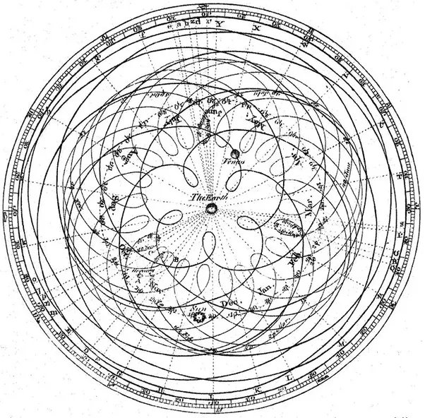
However, as we have seen, 3D-rotors are a three-dimensional concept that does not require the use of “four-dimensional double turns” or “stereographic projection” for visualization. Attempting to visualize quaternions working in 4D to explain 3D turns is a bit like trying to understand the movement of the planets from a geocentric point of view. Those. this approach is too complicated because we look at it from the wrong point of view.
As we have seen, modeling turns as occurring inside planes, rather than around vectors, helps us a lot. For example, squares of basic bivectors give −1 , just like basic quaternions ( mathbfi2= mathbfj2= mathbfk2=−1 ):
( mathbfx mathbfy)2=( mathbfx mathbfy)( mathbfx mathbfy)=−( mathbfy mathbfx)( mathbfx mathbfy)=− mathbfy( mathbfx mathbfx) mathbfy=− mathbfy mathbfy=−1
Multiplying two bivectors on each other gives the third bivector, but in fact it’s trivial, and we don’t need to remember that mathbfi mathbfj= mathbfk :
( mathbfx mathbfy)( mathbfy mathbfz)= mathbfx( mathbfy mathbfy) mathbfz= mathbfx mathbfz
(Notice that we used mathbfx wedge mathbfy= mathbfx mathbfy )
These properties are a consequence of the geometric product, and do not arise from nowhere!
Additional reading
(By the way, in geometric algebra there are not only rotors, but also other cool things!)
- Linear and Geometric Algebra by Macdonald [ link to Amazon ]
An excellent source, very clear and understandable, because it was meant that it would replace the textbook of linear algebra for students. - Geometric Algebra For Computer Science by Dorst et al. [ link to Amazon ]
Excellent source, because programming sometimes allows you to better understand the subject.Note: in this book, the authors make it clear that geometric algebra is slower than quaternions (and the like ...). In fact, it should have approximately the same code (i.e. you should not write code for geometric algebra, creating a generalized struct that can contain all possible types of k-vectors, just write one struct for each type of k-vectors if necessary That is, to replace quaternions, you can write one Bivector structure and one Rotor structure (which is Scalar + Bivector).
Source: https://habr.com/ru/post/429640/
All Articles