Seals vs neural network 2. Or run SqueezeNet v.1.1 on Raspberry Zero in realtime (almost)
Hello!
After writing it was not quite serious and not particularly useful in the practical way of the first part, I was slightly bogged down with conscience. And I decided to finish the job. That is, choose the same implementation of the neural network to run on Rasperry Pi Zero W in real time (of course, as far as possible on such hardware). Run it on the data from real life and highlight the results obtained on Habré.
Caution! There is a workable code under the cut and a little more seal than in the first part. The picture shows the ko and ko respectively.
')

Let me remind you that due to the weakness of the malinki iron, the choice of implementations of the neural network is small. Namely:
1. SqueezeNet.
2. YOLOv3 Tiny.
3. MobileNet.
4. ShuffleNet.
How correct was the choice in favor of SqueezeNet in the first part ? .. To run each of the above mentioned neural networks on its hardware is a rather long event. Therefore, tormented by vague doubts, I decided to google, if someone had asked myself a similar question. It turned out that he asked and investigated it in some detail. Those interested can refer to the source . I will confine myself to the only picture of it:
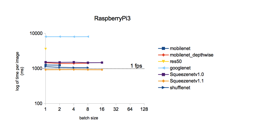
It follows from the picture that the processing time of one image for different models trained on ImageNet is the least time for SqueezeNet v.1.1. We take this as a guide to action. The comparison was not included YOLOv3, but, as I recall, YOLO is more expensive than MobileNet. Those. In speed, it should also give in to SqueezeNet.
Weights and the SqueezeNet topology, trained on the ImageNet dataset (the Caffe framework), can be found on GitHub . Just in case I downloaded both versions so that they could be compared later. Why ImageNet? This set of all available has the maximum number of classes (1000 pieces), so the results of the neural network promise to be quite interesting.
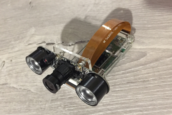
At this time, let's see how Raspberry Zero copes with the recognition of frames from the camera. Here it is, our humble worker of today's post:
I took the source code from Adrian Rosebrock’s blog, mentioned in the first part , namely from here . But I had to significantly plow it up:
1. Replace the model in use with MobileNetSSD with SqueezeNet.
2. Execution of item 1 led to an increase in the number of classes to 1000. But, at the same time, the function of selecting objects with multi-colored frames (SSD functionality) had, alas, to be removed.
3. Remove the argument reception via the command line (for some reason, this puts me at the input of parameters).
4. Remove the VideoStream method, and with it the imutils library, beloved by Adrian. The original method was used to get the video stream from the camera. But with the camera connected to Raspberry Zero, he stupidly did not work, giving out something like “Illegal instruction”.
5. Add the frame rate (FPS) to the recognized picture, rewrite the FPS calculation.
6. Make saving frames to write this post.
On Malinka with Rapbian Stretch OS, Python 3.5.3 and installed via pip3 install OpenCV 3.4.1, the following happened and started:
The code displays on the screen of the monitor connected to the Raspberry, the next recognized frame in this form. At the top of the frame, only the most likely class is displayed.

So, a computer mouse was defined as a mouse with a very high probability. At the same time, images are updated with a frequency of 0.34 FPS (i.e., approximately once every three seconds). It is a bit annoying to hold the camera and wait for the next frame to be processed, but you can live. By the way, if you remove the save frame on the SD card, the processing speed will increase to 0.37 ... 0.38 FPS. Surely, there are other ways to disperse. We will live and see, in any case, leave this question for the next posts.
Separately, I apologize for the white balance. The fact is that the IR camera with the backlight turned on was connected to Rapberry, so most of the frames look rather strange. But the more valuable every hit neural network. Obviously, the white balance on the training set was more correct. In addition, I decided to insert just raw frames so that the reader could see them in the same way as he sees a neural network.
To begin, let's compare the work of SqueezeNet versions 1.0 (on the left frame) and 1.1 (on the right):
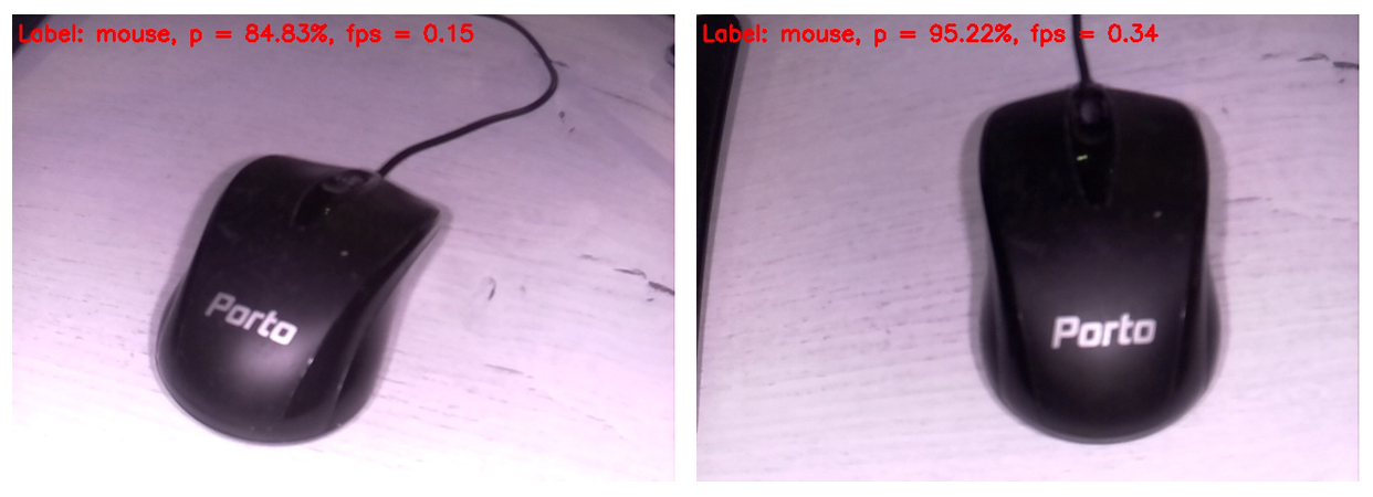
It is seen that version 1.1 runs at two and a quarter times faster than 1.0 (0.34 FPS vs. 0.15). The gain in speed is palpable. Findings on the accuracy of recognition in this example are not worth doing, since the accuracy strongly depends on the position of the camera relative to the object, lighting, glare, shadows, etc.
Due to the significant speed advantage of v1.1 over v.1.0, only SqueezeNet v.1.1 was used in the future. To evaluate the work of the model, I directed the camera at various items thatcame to hand and received the following shots at the output:
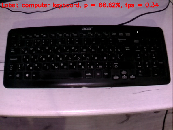
The keyboard is defined worse than the mouse. Perhaps in the training set, most of the keyboards were white.
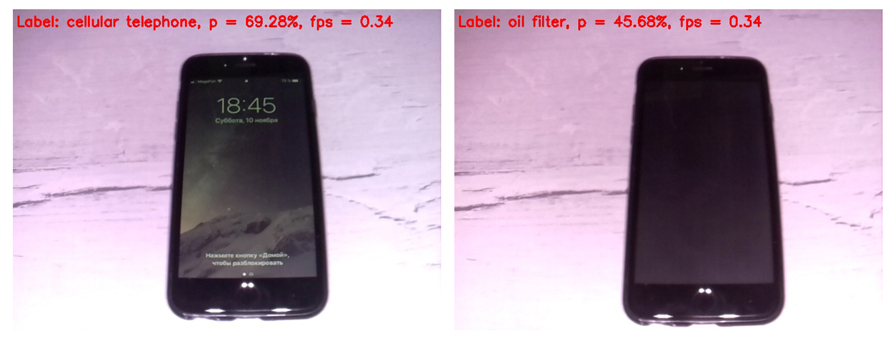
Cell phone is determined pretty well, if you turn on the screen. Cellular with the screen off the neural network for the cell does not count.
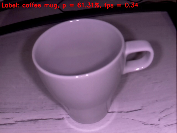
An empty cup is quite well defined as a coffee cup. So far so good.
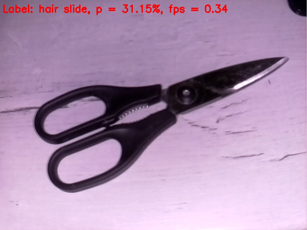
With scissors, the situation is worse, they are stubbornly determined by the network as a hairpin. However, the hit if not in the apple, then at least in the apple tree)
Let's try to put the neural networkpig something tricky. I just got a homemade children's toy. I believe that most readers recognize her as a toy cat. Interestingly, what will our rudimentary artificial intelligence find it?
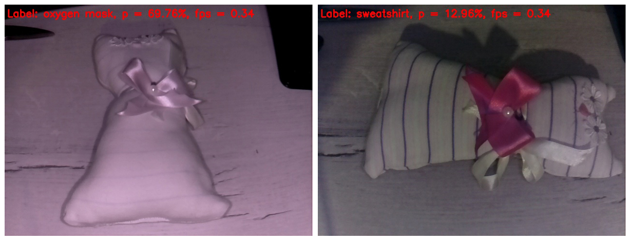
On the frame on the left, the IR illumination erased all the strips from the fabric. As a result, the toy was defined as an oxygen mask with a fairly decent probability. Why not? The shape of the toy really resembles an oxygen mask.
On the frame on the right, I covered the IR illuminator with my fingers, so the stripes appeared on the toy, and the white balance became more believable. Actually, this is the only frame in this post that looks more or less normal. But the neural network such an abundance of details on the image is confusing. She identified the toy as a sweatshirt (sweatshirt). I must say that this, too, does not look like a "finger to the sky." Hitting if not in the "apple tree", then at least in the apple orchard).
Well, we smoothly approached the culmination of our action. The undisputed winner of the fight, thoroughly consecrated in the first post, enters the ring. And it easily takes out the brain of our neural network from the very first frames.

It is curious that the cat practically does not change the position, but each time is determined differently. And in this perspective, it is most similar to a skunk. In second place is the similarity with the hamster. Let's try to change the angle.
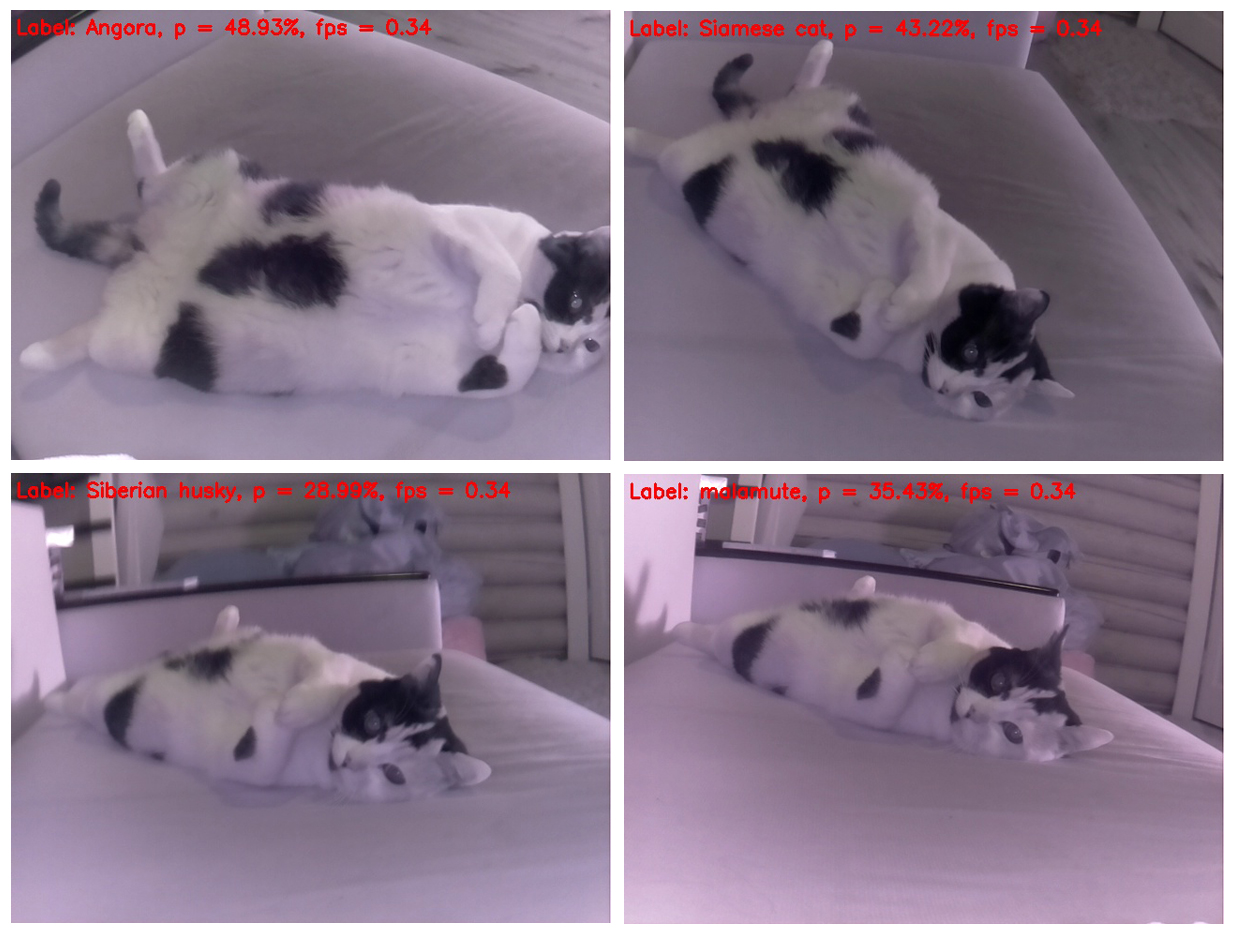
Yeah, if you take a picture of the cat from above, it is determined correctly, but you only have to change the position of the cat's body in the frame a little, for a neural network it becomes a dog - Siberian Husky and Malamute (Eskimo sled dog), respectively.

And this selection is beautiful because a cat of a different breed is defined on each separate frame. And the breed does not repeat)
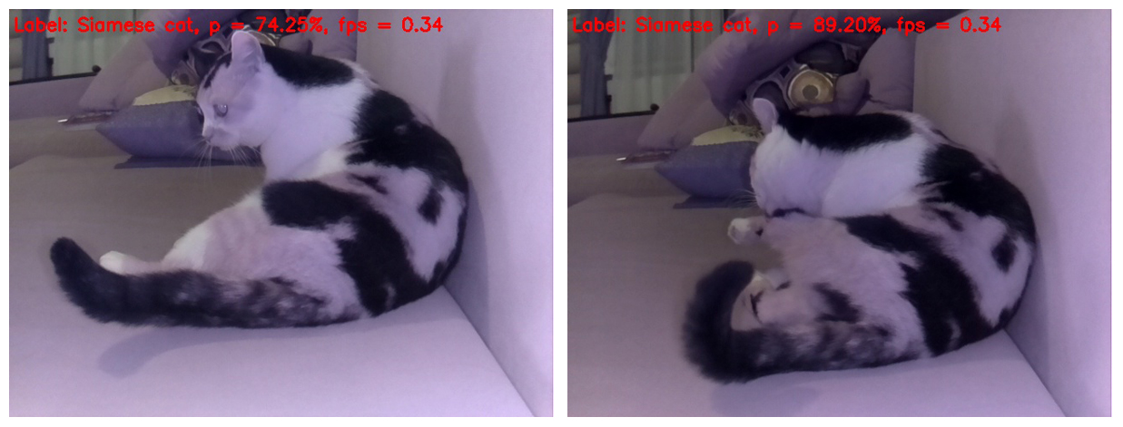
By the way, there are poses in which the neural network becomes obvious that this is still a cat, not a dog. That is, SqueezeNet v.1.1 still managed to show itself even on such a complex object for analysis. Given the success of the neural network in the recognition of objects at the beginning of the test and the recognition of the cat as a cat at the end this time we declare a solid combat draw)
Well, that's all. I suggest everyone to try the proposed code on his raspberry and any animated and inanimate objects that came into view. I will be especially grateful to those who measure FPS on Rapberry Pi B +. I promise to include the results in this post with reference to the person who sent the data. I believe that it should turn out significantly more than 1 FPS!
I hope that the information from this post will be useful to someone for entertainment or educational purposes, and someone, maybe even, will push on new ideas.
All successful work week! And to new meetings)

UPD1: On the Raspberry Pi 3B +, the above script runs at a frequency of 2 with a small FPS.
UPD2: On RPi 3B + with Movidius NCS, the script runs at 6 FPS.
After writing it was not quite serious and not particularly useful in the practical way of the first part, I was slightly bogged down with conscience. And I decided to finish the job. That is, choose the same implementation of the neural network to run on Rasperry Pi Zero W in real time (of course, as far as possible on such hardware). Run it on the data from real life and highlight the results obtained on Habré.
Caution! There is a workable code under the cut and a little more seal than in the first part. The picture shows the ko and ko respectively.
')
Which network to choose?
Let me remind you that due to the weakness of the malinki iron, the choice of implementations of the neural network is small. Namely:
1. SqueezeNet.
2. YOLOv3 Tiny.
3. MobileNet.
4. ShuffleNet.
How correct was the choice in favor of SqueezeNet in the first part ? .. To run each of the above mentioned neural networks on its hardware is a rather long event. Therefore, tormented by vague doubts, I decided to google, if someone had asked myself a similar question. It turned out that he asked and investigated it in some detail. Those interested can refer to the source . I will confine myself to the only picture of it:
It follows from the picture that the processing time of one image for different models trained on ImageNet is the least time for SqueezeNet v.1.1. We take this as a guide to action. The comparison was not included YOLOv3, but, as I recall, YOLO is more expensive than MobileNet. Those. In speed, it should also give in to SqueezeNet.
Implementing the selected network
Weights and the SqueezeNet topology, trained on the ImageNet dataset (the Caffe framework), can be found on GitHub . Just in case I downloaded both versions so that they could be compared later. Why ImageNet? This set of all available has the maximum number of classes (1000 pieces), so the results of the neural network promise to be quite interesting.
At this time, let's see how Raspberry Zero copes with the recognition of frames from the camera. Here it is, our humble worker of today's post:
I took the source code from Adrian Rosebrock’s blog, mentioned in the first part , namely from here . But I had to significantly plow it up:
1. Replace the model in use with MobileNetSSD with SqueezeNet.
2. Execution of item 1 led to an increase in the number of classes to 1000. But, at the same time, the function of selecting objects with multi-colored frames (SSD functionality) had, alas, to be removed.
3. Remove the argument reception via the command line (for some reason, this puts me at the input of parameters).
4. Remove the VideoStream method, and with it the imutils library, beloved by Adrian. The original method was used to get the video stream from the camera. But with the camera connected to Raspberry Zero, he stupidly did not work, giving out something like “Illegal instruction”.
5. Add the frame rate (FPS) to the recognized picture, rewrite the FPS calculation.
6. Make saving frames to write this post.
On Malinka with Rapbian Stretch OS, Python 3.5.3 and installed via pip3 install OpenCV 3.4.1, the following happened and started:
Code here
import picamera from picamera.array import PiRGBArray import numpy as np import time from time import sleep import datetime as dt import cv2 # prototxt = 'models/squeezenet_v1.1.prototxt' model = 'models/squeezenet_v1.1.caffemodel' labels = 'models/synset_words.txt' # rows = open(labels).read().strip().split("\n") classes = [r[r.find(" ") + 1:].split(",")[0] for r in rows] # print("[INFO] loading model...") net = cv2.dnn.readNetFromCaffe(prototxt, model) print("[INFO] starting video stream...") # camera = picamera.PiCamera() camera.resolution = (640, 480) camera.framerate = 25 # camera.start_preview() sleep(1) camera.stop_preview() # raw rawCapture = PiRGBArray(camera) # FPS t0 = time.time() # for frame in camera.capture_continuous(rawCapture, format="bgr", use_video_port=True): # blob frame = rawCapture.array blob = cv2.dnn.blobFromImage(frame, 1, (224, 224), (104, 117, 124)) # blob, net.setInput(blob) preds = net.forward() preds = preds.reshape((1, len(classes))) idxs = int(np.argsort(preds[0])[::-1][:1]) # FPS FPS = 1/(time.time() - t0) t0 = time.time() # , FPS, text = "Label: {}, p = {:.2f}%, fps = {:.2f}".format(classes[idxs], preds[0][idxs] * 100, FPS) cv2.putText(frame, text, (5, 25), cv2.FONT_HERSHEY_SIMPLEX, 0.7, (0, 0, 255), 2) print(text) cv2.imshow("Frame", frame) # Raspberry fname = 'pic_' + dt.datetime.now().strftime('%Y-%m-%d_%H-%M-%S') + '.jpg' cv2.imwrite(fname, frame) # SD key = cv2.waitKey(1) & 0xFF # `q` if key == ord("q"): break # raw rawCapture.truncate(0) print("[INFO] video stream is terminated") # cv2.destroyAllWindows() camera.close() results
The code displays on the screen of the monitor connected to the Raspberry, the next recognized frame in this form. At the top of the frame, only the most likely class is displayed.
So, a computer mouse was defined as a mouse with a very high probability. At the same time, images are updated with a frequency of 0.34 FPS (i.e., approximately once every three seconds). It is a bit annoying to hold the camera and wait for the next frame to be processed, but you can live. By the way, if you remove the save frame on the SD card, the processing speed will increase to 0.37 ... 0.38 FPS. Surely, there are other ways to disperse. We will live and see, in any case, leave this question for the next posts.
Separately, I apologize for the white balance. The fact is that the IR camera with the backlight turned on was connected to Rapberry, so most of the frames look rather strange. But the more valuable every hit neural network. Obviously, the white balance on the training set was more correct. In addition, I decided to insert just raw frames so that the reader could see them in the same way as he sees a neural network.
To begin, let's compare the work of SqueezeNet versions 1.0 (on the left frame) and 1.1 (on the right):
It is seen that version 1.1 runs at two and a quarter times faster than 1.0 (0.34 FPS vs. 0.15). The gain in speed is palpable. Findings on the accuracy of recognition in this example are not worth doing, since the accuracy strongly depends on the position of the camera relative to the object, lighting, glare, shadows, etc.
Due to the significant speed advantage of v1.1 over v.1.0, only SqueezeNet v.1.1 was used in the future. To evaluate the work of the model, I directed the camera at various items that
The keyboard is defined worse than the mouse. Perhaps in the training set, most of the keyboards were white.
Cell phone is determined pretty well, if you turn on the screen. Cellular with the screen off the neural network for the cell does not count.
An empty cup is quite well defined as a coffee cup. So far so good.
With scissors, the situation is worse, they are stubbornly determined by the network as a hairpin. However, the hit if not in the apple, then at least in the apple tree)
Complicate the task
Let's try to put the neural network
On the frame on the left, the IR illumination erased all the strips from the fabric. As a result, the toy was defined as an oxygen mask with a fairly decent probability. Why not? The shape of the toy really resembles an oxygen mask.
On the frame on the right, I covered the IR illuminator with my fingers, so the stripes appeared on the toy, and the white balance became more believable. Actually, this is the only frame in this post that looks more or less normal. But the neural network such an abundance of details on the image is confusing. She identified the toy as a sweatshirt (sweatshirt). I must say that this, too, does not look like a "finger to the sky." Hitting if not in the "apple tree", then at least in the apple orchard).
Well, we smoothly approached the culmination of our action. The undisputed winner of the fight, thoroughly consecrated in the first post, enters the ring. And it easily takes out the brain of our neural network from the very first frames.
It is curious that the cat practically does not change the position, but each time is determined differently. And in this perspective, it is most similar to a skunk. In second place is the similarity with the hamster. Let's try to change the angle.
Yeah, if you take a picture of the cat from above, it is determined correctly, but you only have to change the position of the cat's body in the frame a little, for a neural network it becomes a dog - Siberian Husky and Malamute (Eskimo sled dog), respectively.
And this selection is beautiful because a cat of a different breed is defined on each separate frame. And the breed does not repeat)
By the way, there are poses in which the neural network becomes obvious that this is still a cat, not a dog. That is, SqueezeNet v.1.1 still managed to show itself even on such a complex object for analysis. Given the success of the neural network in the recognition of objects at the beginning of the test and the recognition of the cat as a cat at the end this time we declare a solid combat draw)
Well, that's all. I suggest everyone to try the proposed code on his raspberry and any animated and inanimate objects that came into view. I will be especially grateful to those who measure FPS on Rapberry Pi B +. I promise to include the results in this post with reference to the person who sent the data. I believe that it should turn out significantly more than 1 FPS!
I hope that the information from this post will be useful to someone for entertainment or educational purposes, and someone, maybe even, will push on new ideas.
All successful work week! And to new meetings)
UPD1: On the Raspberry Pi 3B +, the above script runs at a frequency of 2 with a small FPS.
UPD2: On RPi 3B + with Movidius NCS, the script runs at 6 FPS.
Source: https://habr.com/ru/post/429400/
All Articles