Software module for digitizing damaged documents

Optical Character Recognition (OCR) is the process of obtaining printed texts in a digitized format. If you read a classic novel on a digital device or asked a doctor to pick up old medical records through the hospital's computer system, you probably took advantage of OCR.

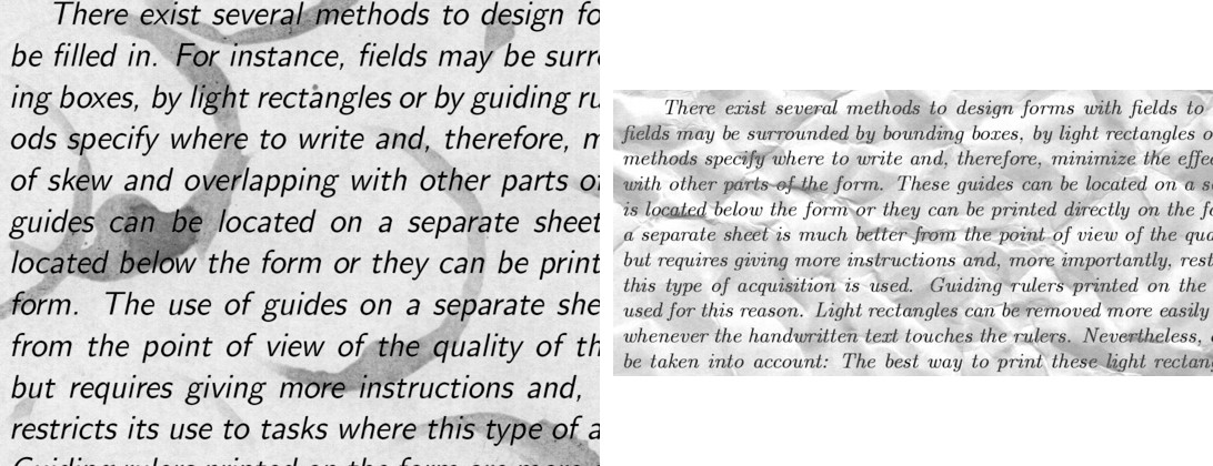
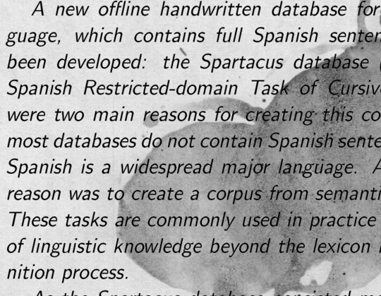
OCR makes previously static content editable, searchable and exchangeable. But many documents that need digitization contain coffee stains, pages with curved corners and many wrinkles retain some printed documents in a non-digitized form.

Everyone has long known that there are millions of old books that are stored in the vaults. The use of these books is prohibited because of their dilapidation and decrepitude, and therefore the digitization of these books is so important.

The paper deals with the task of clearing text from noise, recognizing text in an image and converting it into text format.

For training used 144 pictures. The size may be different, but preferably should be within reason. Pictures must be in PNG format. After reading the image, binarization is used - the process of converting a color image to black and white, that is, each pixel is normalized to the range from 0 to 255, where 0 is black, 255 is white.

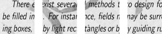
To train a convolutional network, you need more images than there are. It was decided to divide the images into parts. Since the training sample consists of images of different sizes, each image was compressed to 448x448 pixels. The result was 144 images at a resolution of 448x448 pixels. After that, they were all cut into non-overlapping windows measuring 112x112 pixels.

Thus, out of the 144 original images, about 2,304 images were obtained in the training set. But this was not enough. For good learning of the convolution network, more examples are needed. In consequence of this, the best option was to rotate the pictures by 90 degrees, then by 180 and 270 degrees. As a result, an array with the size [16,112,112,1] is fed to the input of the network. Where 16 is the number of images, 112 is the width and height of each image, 1 is the color channels. It turned out 9216 examples for learning. This is enough to train a convolutional network.

Each image has a size of 112x112 pixels. If the size is too large, the computational complexity will increase, respectively, the limitations on the speed of response will be violated, the determination of the size in this problem is solved by the selection method. If you select a size that is too small, the network will not be able to identify key features. Each image has a black and white format, so it is divided into 1 channel. Color images are divided into 3 channels: red, blue, green. Since we have black and white images, the size of each image is 112x122x1 pixels.

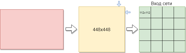
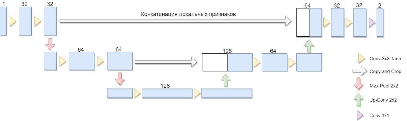
First of all, it is necessary to train a convolutional neural network on the harvested, processed images. For this task, the U-Net architecture was chosen.

A reduced version of the architecture was selected, consisting of only two blocks (the original version of four). An important consideration was the fact that a large class of well-known binarization algorithms is explicitly expressed in such an architecture or a similar architecture (as an example, we can take a modification of the Niblack algorithm with the replacement of the standard deviation by the mean deviation modulus, in this case the network is especially simple).

The advantage of this architecture is that you can create a sufficient amount of training data from a small number of source images for network training. At the same time, the network has a relatively small number of weights due to its convolutional architecture. But there are some nuances. In particular, the artificial neural network used, strictly speaking, does not solve the problem of binarization: it assigns to each pixel of the original image a certain number from 0 to 1, which characterizes the degree of belonging of this pixel to one of the classes (meaningful filling or background) and still convert to final binary answer. [one]

U-Net consists of a compressing and unclamping path and “forwarding” between them. The compression path, in this architecture, consists of two blocks (in the original version of four). In each block, there are two bundles with a 3x3 filter (using the Tanh activation function after folding) and a pooling with a 2x2 filter size in increments of 2. The number of channels at each step down is doubled.

Splitting path also consists of two blocks. Each of them consists of a “sweep” with a 2x2 filter size, halving the number of channels, concatenation with a corresponding truncated feature map from a compression path (“forwarding”), and two bundles with a 3x3 filter (using the Tanh activation function after folding). Next, on the last layer, the 1x1 convolution (using the Sigmoid activation function) to produce an output, flat image. Note that clipping the feature map during concatenation is significant due to the loss of boundary pixels at each convolution. Adam was chosen as the method of stochastic optimization.

In general, the architecture is a sequence of layers of convolution + pooling, which reduce the spatial resolution of the image, then increase it by combining with the image data in advance and passing it through other layers of the convolution. Thus, the network serves as a kind of filter. [2]

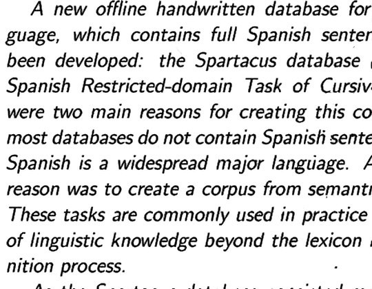
The test sample consisted of similar images, the differences were only in the texture of noise and in the text. Network testing took place on this image.

The output of the convolutional neural network is an array of numbers with a size [16,112,112,1]. Each number is a separate pixel processed by the network. The images have a format of 112x112 pixels, as before, it was cut into pieces. She needs to betray the original look. We merge the obtained images into one part, as a result, the picture has the format of 448x448. Then we multiply each number in the array by 255 to get the range from 0 to 255, where 0 is black, 255 is white. We return the image to its original size, as before, it was compressed. The result is a picture below in the picture.

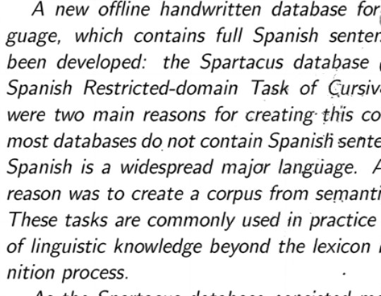
In this example, it is clear that the convolutional network has coped with the majority of noisiness and has shown itself to work. But it is clearly noticeable that the picture has become duller and the missed noises are visible. In the future, this may affect the accuracy of text recognition.

Based on this fact, it was decided to use another neural network - a multilayer perceptron. In the expected result, the network should make the text in the image clearer and remove the noisiness missed by the convolutional neural network.

An image that has already been processed by a convolutional network is sent to the input of the multilayer perceptron. In this case, the training sample for this network will differ from the sample for the convolutional network, since the networks process the image differently. A convolutional network is considered to be the main network and removes most of the noise in the image, while the multi-layer perceptron processes what the convolutional failed.
Here are some examples from a training sample for a multilayer perceptron.

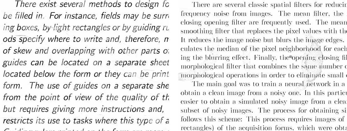
The image data was obtained by processing the training sample for the convolutional network with a multilayer perceptron. At the same time, the perceptron was trained on the same sample, but on a small number of examples and a small number of epochs.

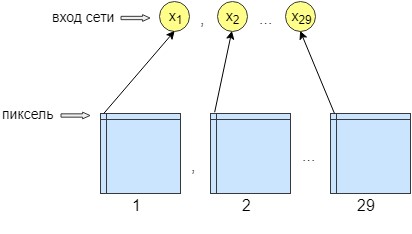
For perceptron training, 36 images were processed. The network is trained pixel-by-pixel, that is, one pixel from the image is sent to the input of the network. At the output of the network we also get one output neuron - one pixel, that is, the response of the network. To increase the processing accuracy, 29 input neurons were made. And on the image obtained after processing by the convolutional network, 28 filters are superimposed. The result is 29 images with different filters. We send one pixel from each 29 images to the network input and only one pixel is received at the network output, that is, the network response.

This was done for better learning and networking. After that, the network began to increase the accuracy and contrast of the image. It also clears minor errors that could not clear the convolutional network.

As a result, the neural network has 29 input neurons, one pixel from each image. After the experiments, it was found that only one hidden layer is needed, in which there are 500 neurons. Outlet at the network one. Since the learning took place pixel by pixel, the network was accessed n * m times, where n is the width of the image, and m is the height, respectively.

After image processing by successively two neural networks, the main thing that remains is to recognize the text. For this, a ready-made solution was taken, namely the Pytesseract Python library. Pytesseract does not provide true Python bindings. Rather, it is a simple wrapper for the tesseract binary file. At the same time tesseract is installed separately on the computer. Pytesseract saves the image to a temporary file on disk, then calls the tesseract binary file and writes the result to a file.

This wrapper is developed by Google and is free and free to use. It can be used both in their own and for commercial purposes. The library works without an internet connection, supports many languages ​​for recognition and impresses with its speed. Its application can be found in various popular applications.

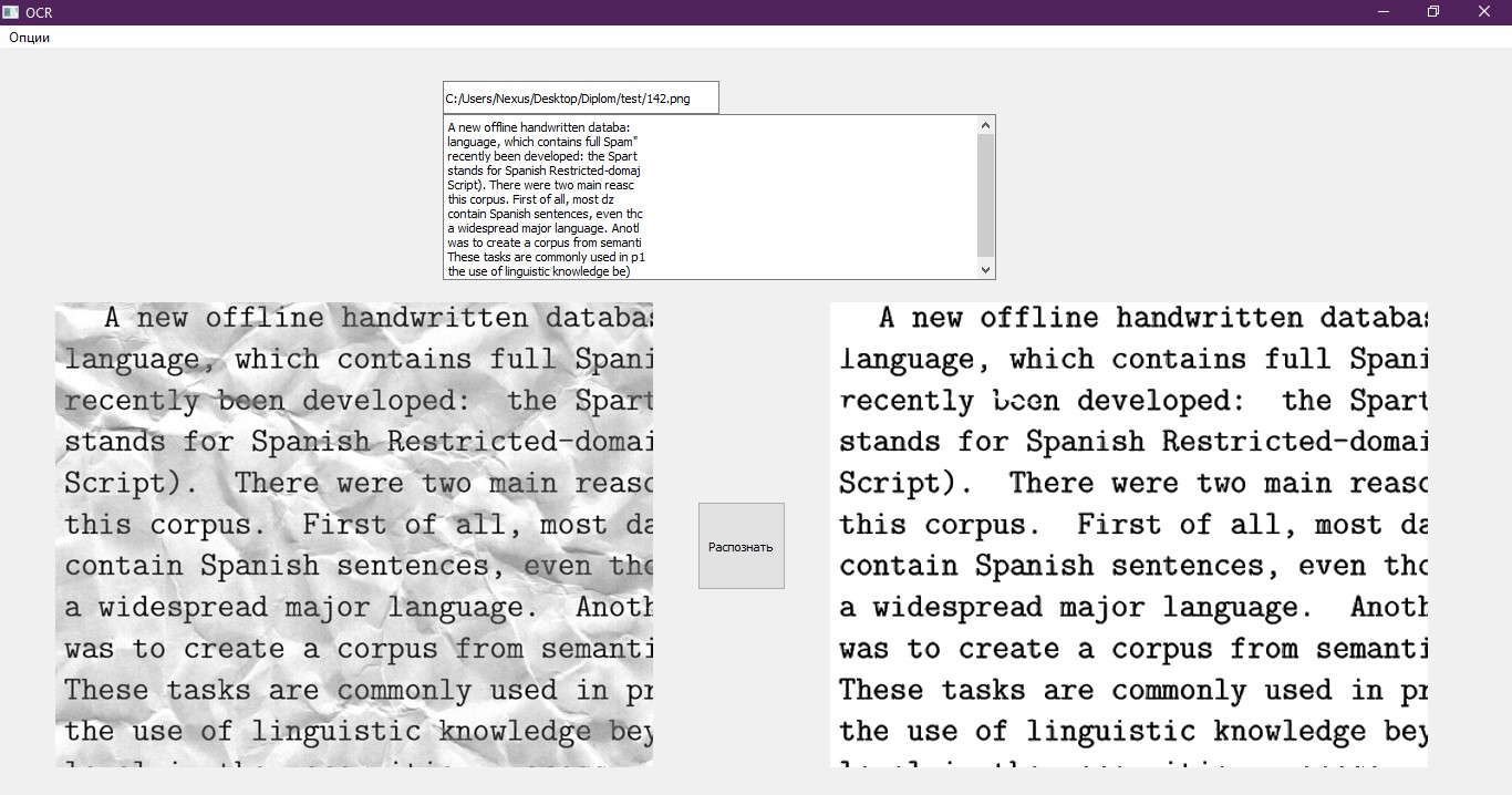
The last item left is to write the recognized text to a file in a format suitable for its processing. We use for this the usual notebook, which opens, after the completion of the program. Also, the text is displayed on the test interface. An illustrative example of the interface.

Bibliography:

1. The history of victory in the international competition for the recognition of documents of the SmartEngines company team [Electronic resource]. Access mode: https://habr.com/company/smartengines/blog/344550/
2. Image segmentation using neural network: U-Net [Electronic resource]. Access mode: http://robocraft.ru/blog/machinelearning/3671.html

> Repository on github